
示例成果
两个示例项目,从输入到论文
两份真实交付成果。选择一个项目,依次查看六个阶段:输入文件、生成的代码、运行过程、全部结果、PDF 阅读器中的论文稿件,以及排版好的 IEEE 论文。点击任意页面或图表可放大。
正在加载 PDF… 0%
一切从构想文档开始,连同方案、参考论文和数据集放在同一个项目文件夹里。写任何内容之前,每一项都会先被读取并评分。
- 构想 PDF,9 页手写
- 方案 DOCX
- 参考论文,16 篇 PDF
- FruitNet 和 FruitQ 数据集
构想文档是起点。在阅读器中可以翻看全部 9 页手写内容。
"""MLRI-Net project hub (tkinter GUI).

* "Run Full Pipeline & Show Graphs" runs every stage for the selected dataset(s)
  on a background thread, then shows all graphs in the built-in gallery.
* Every stage can also be run on its own, as can the sample case study, the
  self-checks and the demo.
* Settings (data percentage, per-class cap, epochs, ...) are saved to run_settings.json.

Start:  python main.py
"""
import os
import queue
import random
import subprocess
import sys
import threading
import tkinter as tk
import traceback
from pathlib import Path
from tkinter import messagebox, scrolledtext, ttk

from PIL import Image, ImageTk

import run_config as cfg
from data_loader import discover_datasets
from feature_cache_builder import PipelineCancelled
from full_pipeline_runner import STAGE_ORDER, STAGE_TITLES, run_full_pipeline
from project_paths import (CODE_DIR, EXPERIMENTAL_OUTPUT_DIR, PARAMETERS_DIR, RESULTS_DIR, SAMPLE_CASE_STUDY_DIR,
                           ensure_output_folders)

ACCENT = "#882255"
PANEL_BG = "#F7F4F2"
THUMB = 230


def open_folder(path):
    path = Path(path)
    path.mkdir(parents=True, exist_ok=True)
    if sys.platform.startswith("win"):
        os.startfile(str(path))                                  # noqa: S606 (Windows only)
    elif sys.platform == "darwin":
        subprocess.Popen(["open", str(path)])
    else:
        subprocess.Popen(["xdg-open", str(path)])


class GraphGallery(ttk.Frame):
    """Scrollable grid of result graphs; click a thumbnail to enlarge it."""

    def __init__(self, master):
        super().__init__(master)
        top = ttk.Frame(self)
        top.pack(fill="x", pady=(4, 2))
        ttk.Label(top, text="Show:").pack(side="left", padx=(6, 2))
        self.filter = ttk.Combobox(top, state="readonly", width=34)
        self.filter.pack(side="left")
        self.filter.bind("<<ComboboxSelected>>", lambda _e: self.refresh())
        ttk.Button(top, text="Reload graphs", command=self.refresh).pack(side="left", padx=6)
        self.count_label = ttk.Label(top, text="")
        self.count_label.pack(side="left", padx=6)
        self.canvas = tk.Canvas(self, background="white", highlightthickness=0)
        scroll = ttk.Scrollbar(self, orient="vertical", command=self.canvas.yview)
        self.inner = tk.Frame(self.canvas, background="white")
        self.inner.bind("<Configure>", lambda _e: self.canvas.configure(scrollregion=self.canvas.bbox("all")))
        self.canvas.create_window((0, 0), window=self.inner, anchor="nw")
        self.canvas.configure(yscrollcommand=scroll.set)
        self.canvas.pack(side="left", fill="both", expand=True)
        scroll.pack(side="right", fill="y")
        self.canvas.bind_all("<MouseWheel>", lambda e: self.canvas.yview_scroll(int(-e.delta / 120), "units"))
        self.canvas.bind_all("<Button-4>", lambda _e: self.canvas.yview_scroll(-1, "units"))
…
"""Proposed method - MLRI-Net (Mean Squared LogCosh loss based Residual Inception Network).
Pipeline (context.docx Sec. 3): CIEWF -> DLNet -> CutMix/MixUp -> {f1 CS-LMP, f2 ResNeXt-101}
-> MLRI-Net -> fruit type + fruit grade -> XAI.
Architecture (Sec. 3.6):
image branch : segmented image Sm (128x128) -> frozen ResNet18 conv1..layer3 (cached)
-> trainable layer4 -> SE channel attention (residual) -> inception (1024 ch) -> GAP
fusion : [1024 image | 256 from f1 CS-LMP | 256 from f2 ResNeXt-101] = 1536-D
heads : FC1 (1024) -> FC2 (128) -> fruit-type head and grade head
loss : L_Tot = 0.5 RMSLE + 0.5 LogCosh on softmax outputs, summed over both heads
optimiser : Adam (beta1 0.9, beta2 0.999, eps 1e-8), lr 1e-3, ReduceLROnPlateau, early stopping
Ablation variants (Sec. 4.7.2) reuse the class with a different configuration:
without DLNet -> image branch, f1 and f2 computed on the CIEWF image (no background isolation)
without augmentation -> no CutMix / MixUp
"""
import torch
import torch.nn as nn
import run_config as cfg
from comparison_method_interface import NeuralTwoHeadMethod
from loss_rmsle_logcosh import MeanSquaredLogCoshLoss
from rai_net_blocks import RAIImageBranch, TwoHeadClassifier
from texture_features_cslmp import CSLMP_DIM
class MLRINet(nn.Module):
def __init__(self, n_types, n_grades, cslmp_dim=CSLMP_DIM, resnext_dim=1000, proj=256, dropout=None):
super().__init__()
dropout = cfg.DROPOUT if dropout is None else dropout
self.image_branch = RAIImageBranch()
self.cslmp_proj = nn.Sequential(nn.Linear(cslmp_dim, proj), nn.ReLU(inplace=True), nn.Dropout(dropout))
self.resnext_proj = nn.Sequential(nn.Linear(resnext_dim, proj), nn.ReLU(inplace=True), nn.Dropout(dropout))
self.classifier = TwoHeadClassifier(RAIImageBranch.out_dim + 2 * proj, n_types, n_grades,
fc1=1024, fc2=128, dropout=dropout)
def forward(self, layer3_maps, vectors, return_maps=False):
f1, f2 = vectors
if return_maps:
image_vec, maps = self.image_branch(layer3_maps, return_maps=True)
else:
image_vec = self.image_branch(layer3_maps)
fused = torch.cat([image_vec, self.cslmp_proj(f1), self.resnext_proj(f2)], dim=1)
type_logits, grade_logits, embedding = self.classifier(fused)
if return_maps:
return type_logits, grade_logits, embedding, maps
return type_logits, grade_logits, embedding
class MLRINetMethod(NeuralTwoHeadMethod):
key = "mlri_net"
display_name = "MLRI-Net (proposed)"
source = "Proposed method (context.docx Sec. 3)"
map_key = "layer3_seg"
vector_keys = ("cslmp_seg", "resnext_seg")
augment = "mix"
default_batch_size = None # -> run_config.BATCH_SIZE at run time
def build_model(self):
return MLRINet(self.n_types, self.n_grades)
def build_optimizer(self, model):
params = [p for p in model.parameters() if p.requires_grad]
return torch.optim.Adam(params, lr=cfg.LEARNING_RATE, betas=(cfg.ADAM_BETA1, cfg.ADAM_BETA2),
eps=cfg.ADAM_EPSILON)
def loss(self):
return MeanSquaredLogCoshLoss()
…"""Building blocks of RAI-Net (Residual-Attention-Inception Network).
Source: Maurya et al., "RAI-Net: Tomato Plant Disease Classification Using
Residual-Attention-Inception Network" (IEEE Access 2025), Sec. IV, Fig. 2:
ResNet18 (fine-tuned last layers) -> 512x4x4 maps
-> channel attention (squeeze-and-excitation), applied residually: y_CA = CA(x) + x (Eq. 8)
-> inception module, concat of 1x1 | 1x1-3x3 | 1x1-5x5 | maxpool-1x1 (Eq. 9) -> 1024x4x4
-> global average pooling -> FC1 -> FC2 (128) -> classes
"""
import torch
import torch.nn as nn
from pretrained_backbones import pretrained_resnet18_layer4
class SqueezeExcitationAttention(nn.Module):
"""Eqs. (1)-(5): F_avg -> conv + ReLU -> conv -> sigmoid = M_c; F_hat = F * M_c."""
def __init__(self, channels=512, reduction=16):
super().__init__()
self.pool = nn.AdaptiveAvgPool2d(1)
self.reduce = nn.Conv2d(channels, channels // reduction, 1)
self.expand = nn.Conv2d(channels // reduction, channels, 1)
self.detach_gate = False # True while computing LRP (gate treated as constant)
def forward(self, x):
gate = torch.sigmoid(self.expand(torch.relu(self.reduce(self.pool(x)))))
if self.detach_gate:
gate = gate.detach()
return x * gate + x # Eq. (8): y_CA = CA(x) + x
def _conv_bn_relu(cin, cout, k):
return nn.Sequential(nn.Conv2d(cin, cout, k, padding=k // 2, bias=False),
nn.BatchNorm2d(cout), nn.ReLU(inplace=True))
class InceptionModule(nn.Module):
"""Eq. (9): multi-scale branches concatenated along channels (512 -> 1024)."""
def __init__(self, cin=512, branch=256):
super().__init__()
self.b1 = _conv_bn_relu(cin, branch, 1)
self.b3 = nn.Sequential(_conv_bn_relu(cin, branch // 2, 1), _conv_bn_relu(branch // 2, branch, 3))
self.b5 = nn.Sequential(_conv_bn_relu(cin, branch // 4, 1), _conv_bn_relu(branch // 4, branch, 5))
self.bp = nn.Sequential(nn.MaxPool2d(3, stride=1, padding=1), _conv_bn_relu(cin, branch, 1))
def forward(self, x):
return torch.cat([self.b1(x), self.b3(x), self.b5(x), self.bp(x)], dim=1)
class RAIImageBranch(nn.Module):
"""Trainable part of RAI-Net on top of the frozen layer3 maps (256x8x8 -> 1024-D)."""
out_dim = 1024
def __init__(self):
super().__init__()
self.layer4 = pretrained_resnet18_layer4() # residual blocks, ImageNet initialised
self.attention = SqueezeExcitationAttention(512)
self.inception = InceptionModule(512, 256)
self.pool = nn.AdaptiveAvgPool2d(1)
def forward(self, layer3_maps, return_maps=False):
l4 = self.layer4(layer3_maps)
att = self.attention(l4)
inc = self.inception(att)
pooled = torch.flatten(self.pool(inc), 1)
if return_maps:
return pooled, {"layer4": l4, "attention": att, "inception": inc}
…"""Stage 3.2 - Contextual Image Enhancement Wiener Filter (CIEWF).
Source: Sudhakar et al., "High-performance parallel multi-scale attention network
with explainable AI for intelligent diagnosis of leaf diseases in agricultural
systems", p. 5, Eqs. (1)-(3):
CIEWF[I(x1,x2)] = alpha + (beta^2 - beta_n^2) / beta^2 * (I(x1,x2) - alpha)
alpha = local mean over the surrounding window s
beta^2 = local variance over s, beta_n^2 = noise variance
This is a locally adaptive (Lee / Wiener) filter. In flat regions the local
variance is close to the noise variance, so the pixel is pulled to the local
mean (noise removed). On edges the variance is large, so the pixel is kept
(detail preserved). The paper says CIEWF "selects the most suitable window"
but gives no size, so each image is filtered with every candidate window in
CIEWF_WINDOWS and the window that removes the most noise while keeping at
least half of the edge energy is kept.
"""
import cv2
import numpy as np
from skimage.metrics import peak_signal_noise_ratio, structural_similarity
import run_config as cfg
def wiener_filter_channel(channel, window, noise_variance=None):
"""Apply Eq. (1) to one float channel in [0, 1]."""
alpha = cv2.blur(channel, (window, window)) # local mean, Eq. (2)
beta_sq = cv2.blur(channel * channel, (window, window)) - alpha ** 2 # local variance, Eq. (3)
beta_sq = np.maximum(beta_sq, 0.0)
if noise_variance is None: # beta_n^2 estimate
noise_variance = float(beta_sq.mean())
gain = np.maximum(beta_sq - noise_variance, 0.0) / np.maximum(beta_sq, noise_variance + 1e-12)
return alpha + gain * (channel - alpha)
def estimate_noise_sigma(gray):
"""Immerkaer's fast noise estimate (sigma) of a float grey image in [0, 1]."""
kernel = np.array([[1, -2, 1], [-2, 4, -2], [1, -2, 1]], dtype=np.float32)
conv = cv2.filter2D(gray.astype(np.float32), -1, kernel)
h, w = gray.shape
return float(np.sqrt(np.pi / 2.0) * np.abs(conv[1:-1, 1:-1]).sum() / (6.0 * (w - 2) * (h - 2)))
def _edge_energy(gray):
return float(cv2.Laplacian(gray.astype(np.float32), cv2.CV_32F).var()) + 1e-12
def enhance_image_ciewf(rgb_uint8, windows=None):
"""Enhance one RGB uint8 image. Returns (enhanced uint8, info dict)."""
windows = windows or cfg.CIEWF_WINDOWS
image = rgb_uint8.astype(np.float32) / 255.0
gray_in = cv2.cvtColor(image, cv2.COLOR_RGB2GRAY)
edge_in = _edge_energy(gray_in)
best = None
for window in windows:
out = np.stack([wiener_filter_channel(image[..., c], window) for c in range(3)], axis=-1)
out = np.clip(out, 0.0, 1.0)
gray_out = cv2.cvtColor(out, cv2.COLOR_RGB2GRAY)
noise = estimate_noise_sigma(gray_out)
edge_keep = _edge_energy(gray_out) / edge_in
# Prefer the lowest residual noise among windows that keep >= 50 % edge energy.
key = (edge_keep < 0.5, noise)
if best is None or key < best[0]:
best = (key, window, out, noise, edge_keep)
_, window, out, noise, edge_keep = best
enhanced = (out * 255.0 + 0.5).astype(np.uint8)
info = {
"ciewf_window": window,
"noise_sigma_before": estimate_noise_sigma(gray_in),
…EasySeer 把项目写成若干个独立的 Python 文件,外加一个主程序。可以打开任意文件阅读,也可以在对话中问它做了什么。
- 项目内容
- 48 个 Python 文件,另有 requirements 和 readme
- 展示
- 四个真实文件的开头几行
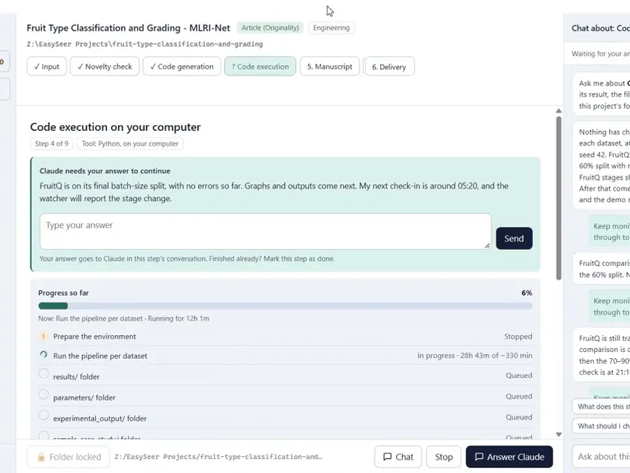
代码在你自己的电脑上运行。所有文件、日志和结果都保存在项目文件夹里,没有任何隐藏。
- 数据集
- FruitNet 和 FruitQ
- 对比方法
- 五种基线方法
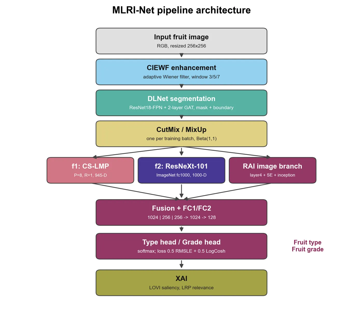
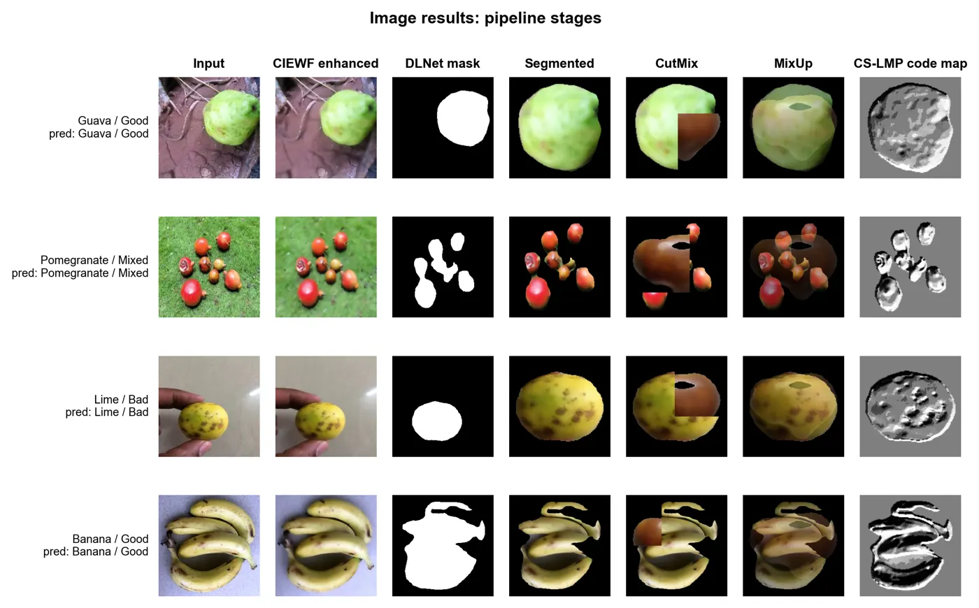
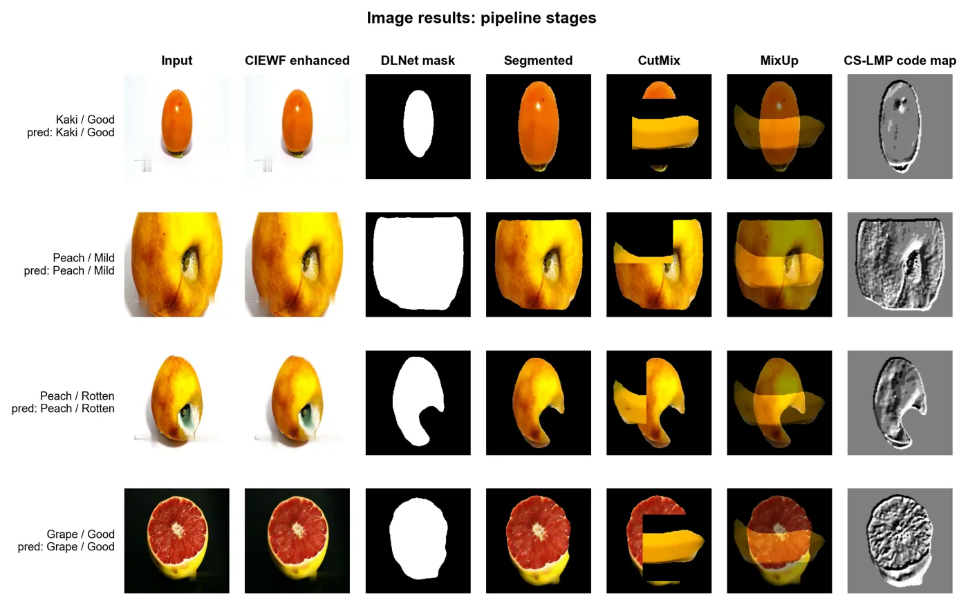
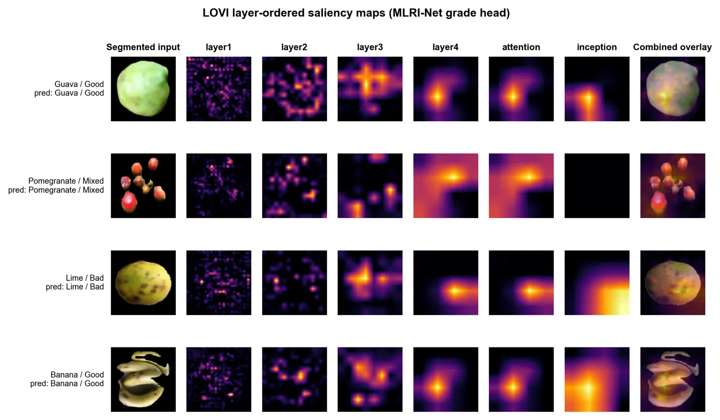
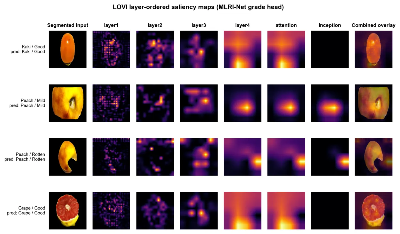
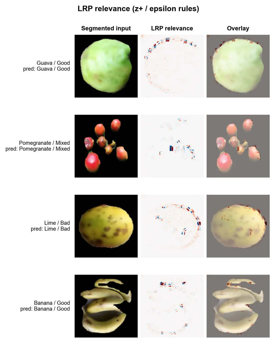
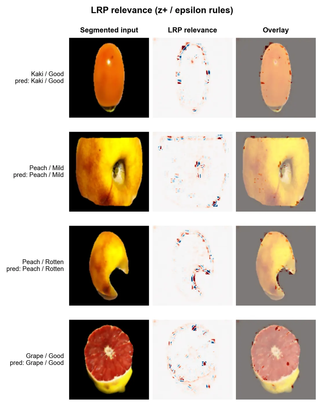
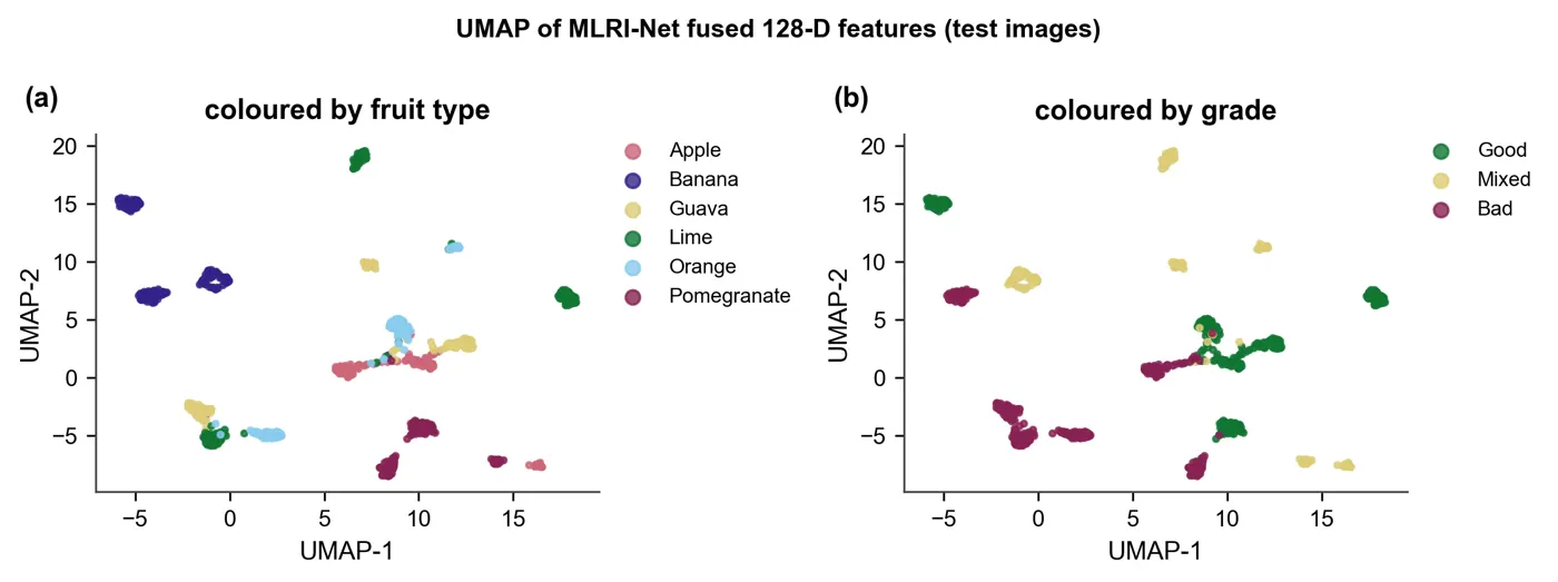
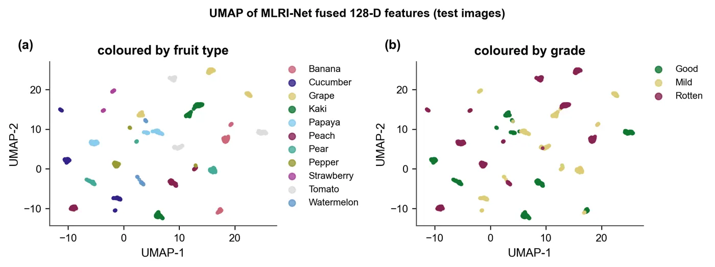
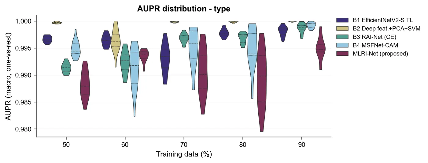
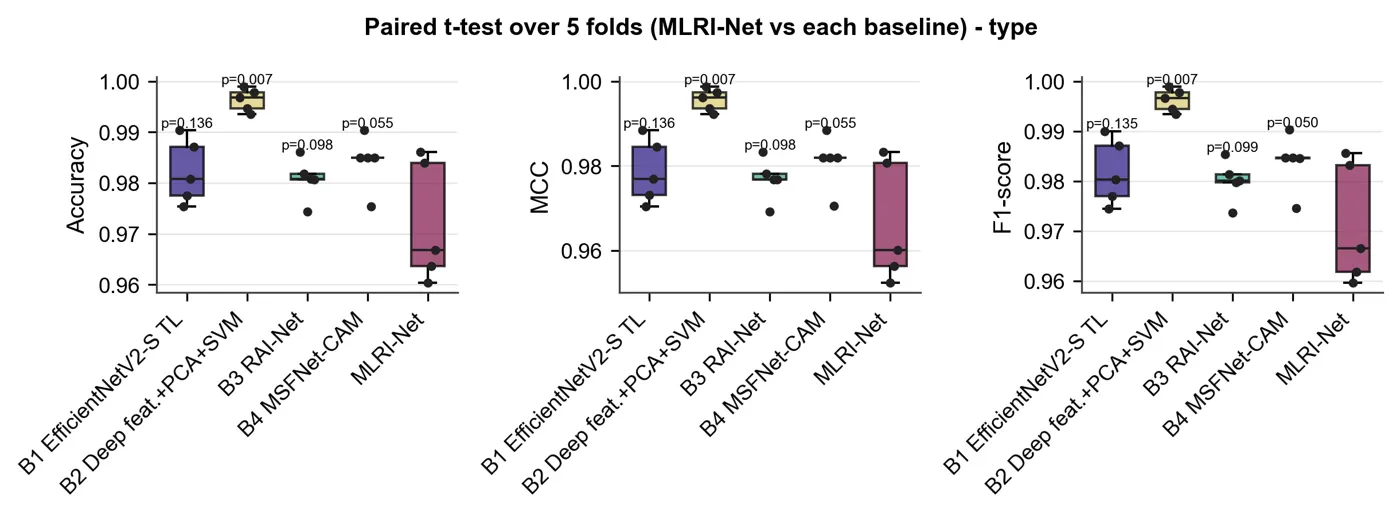
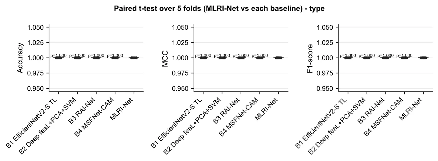
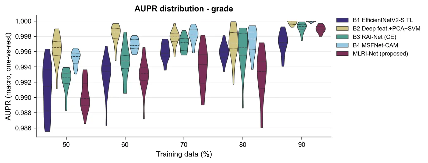
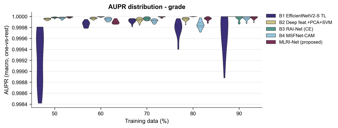
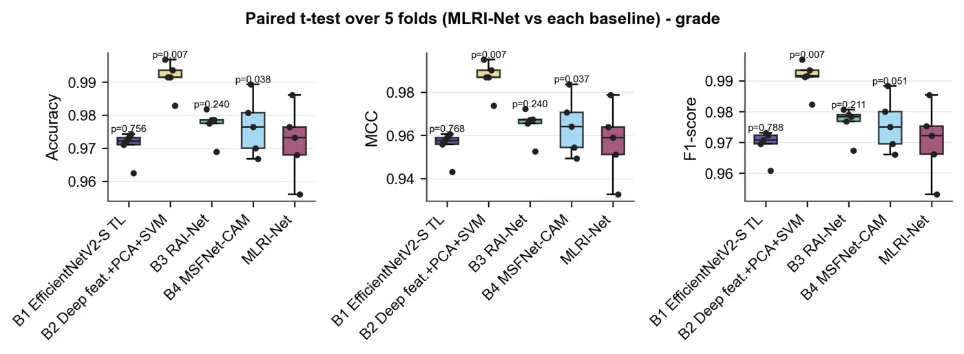
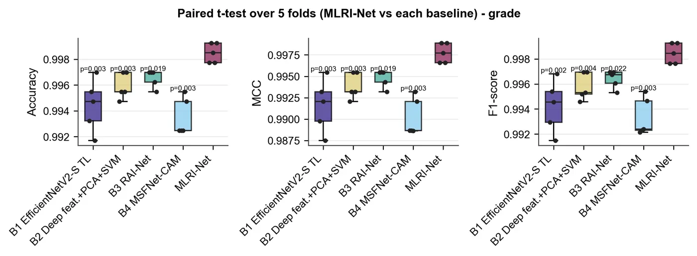
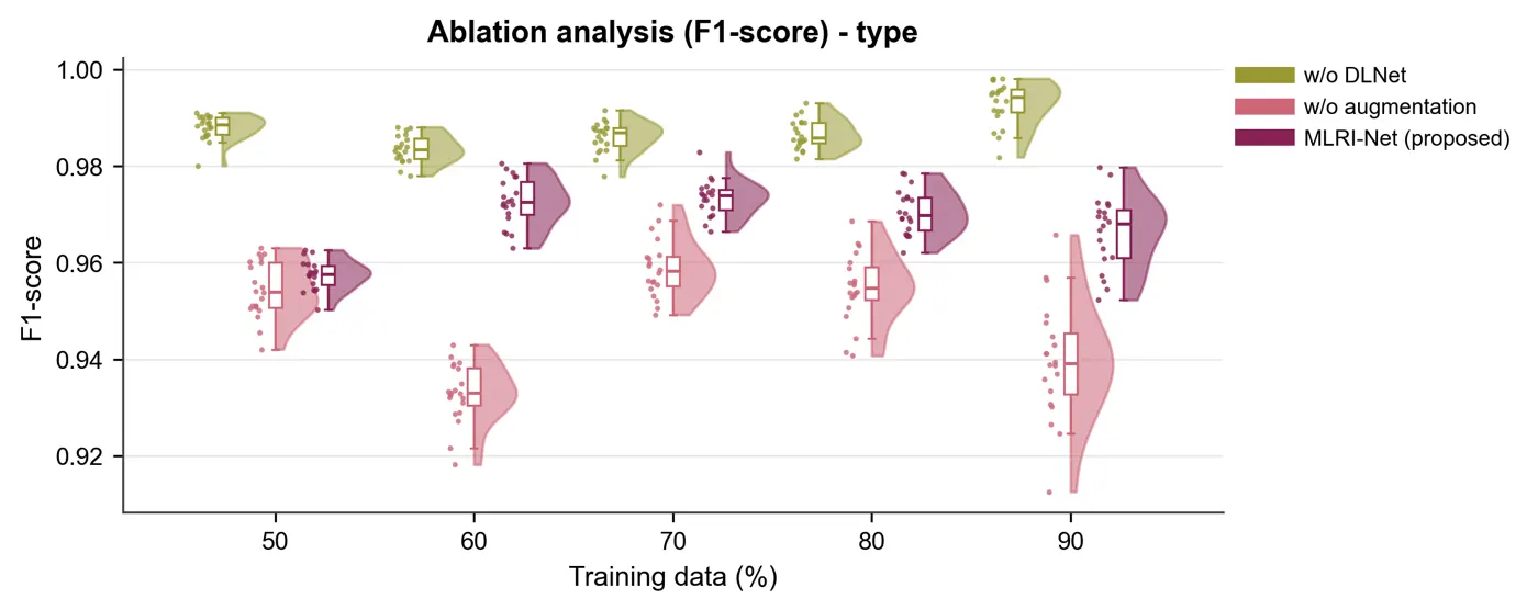
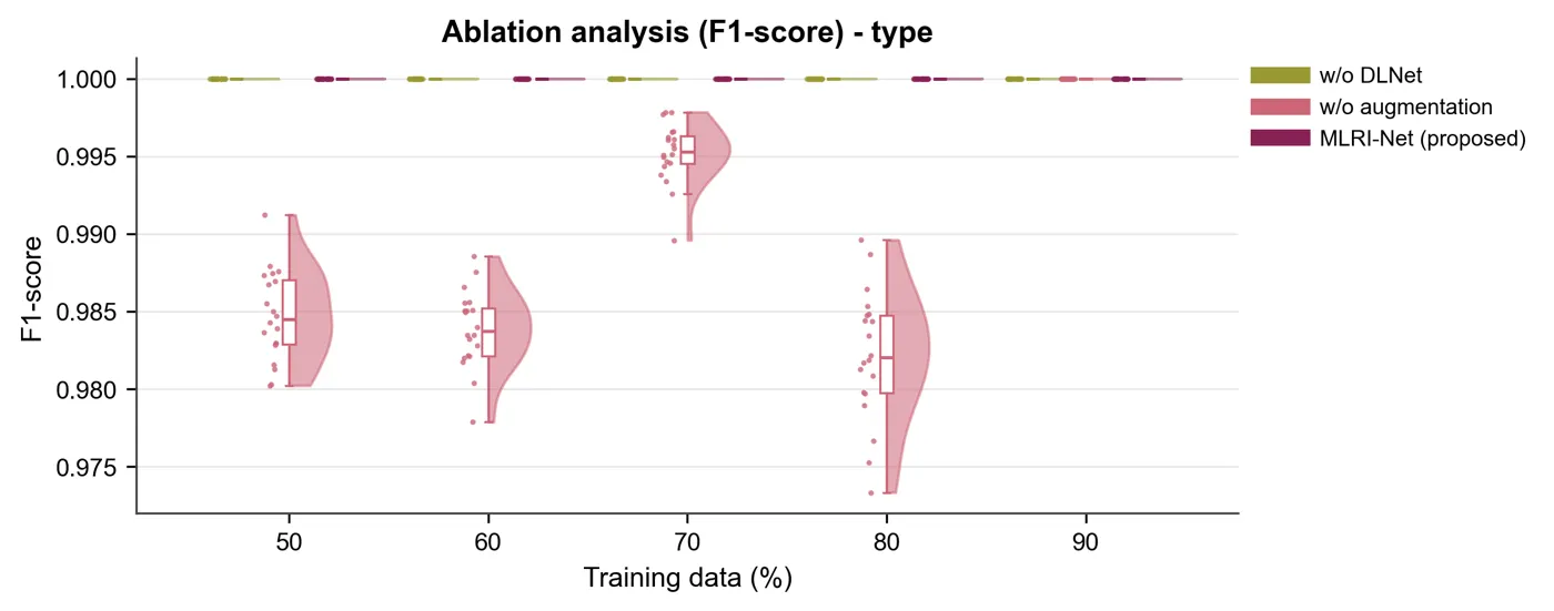
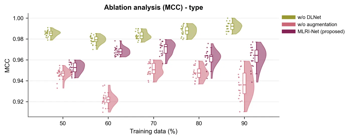
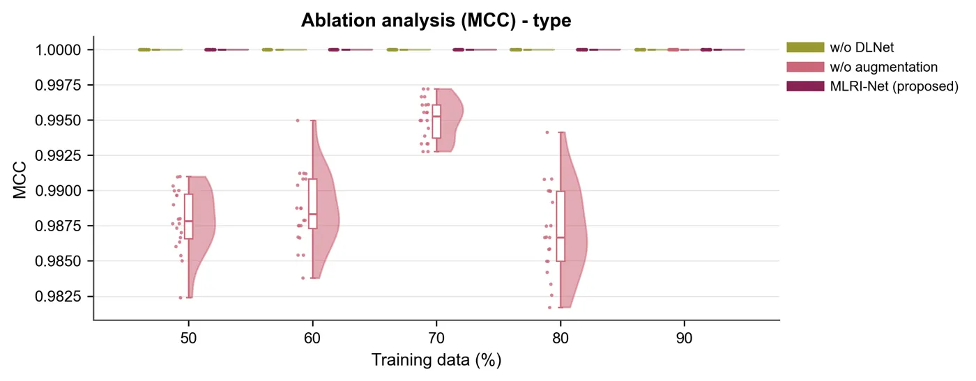
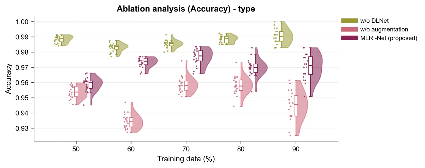
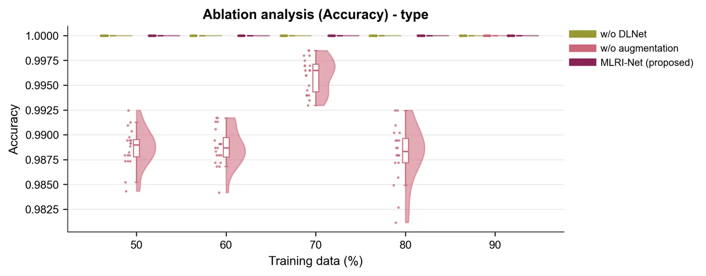
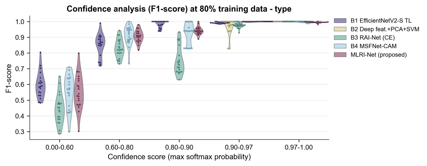
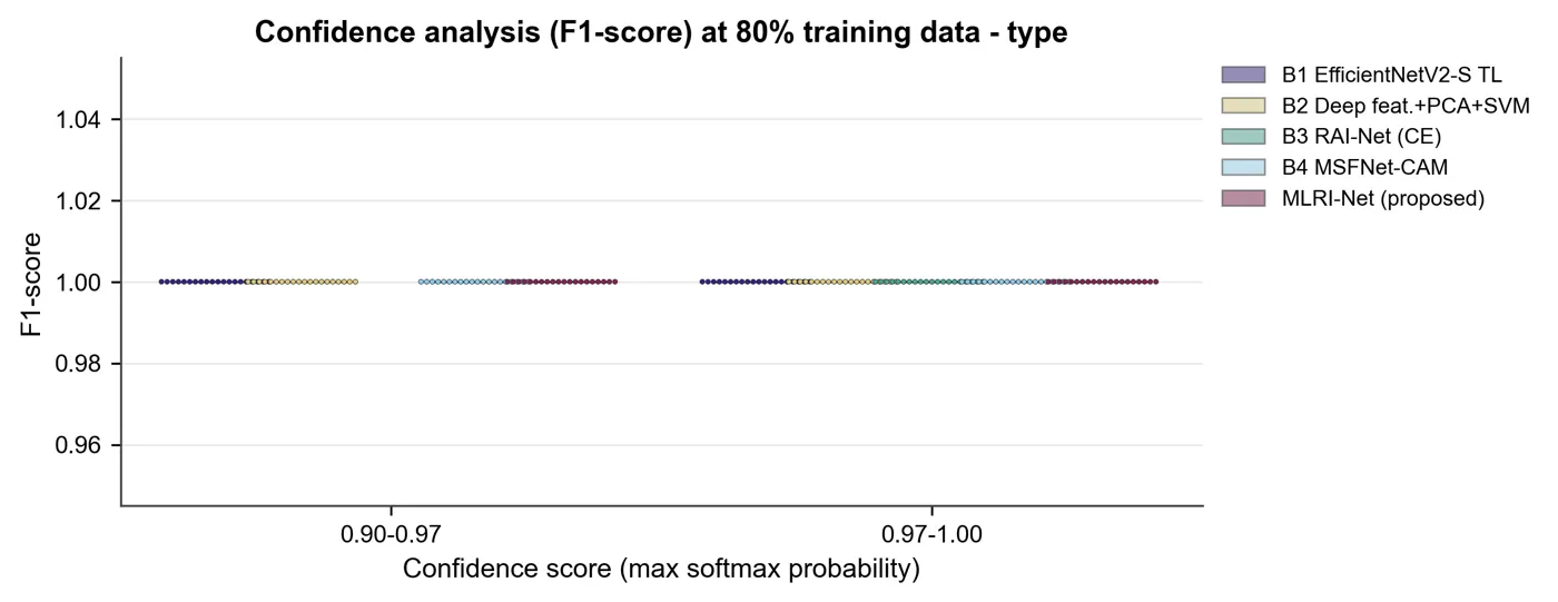
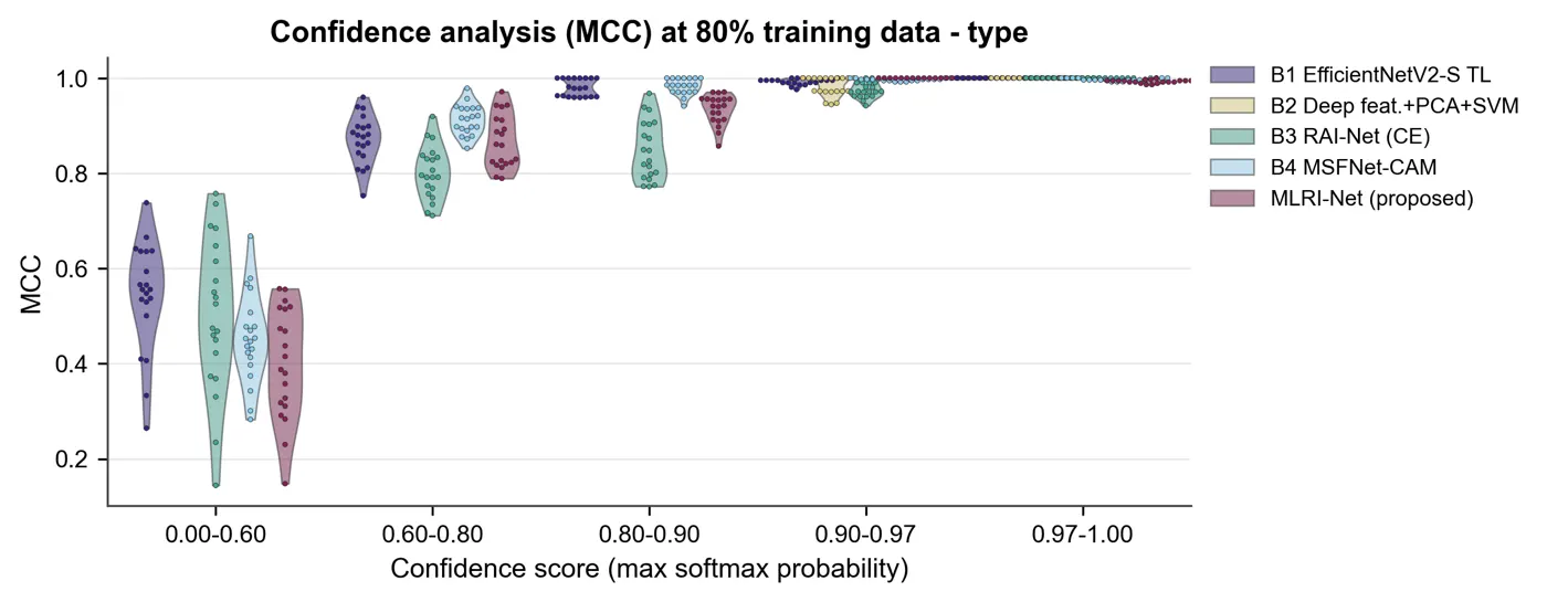
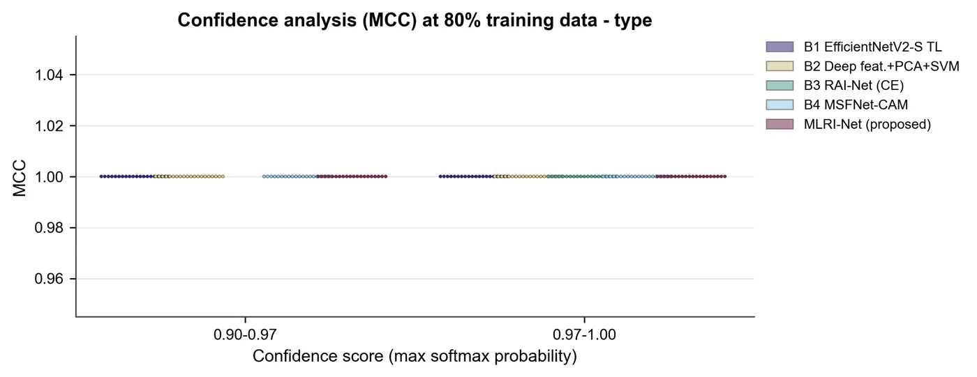
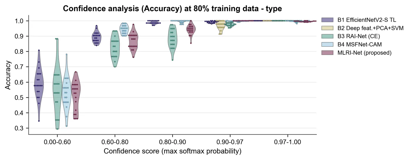
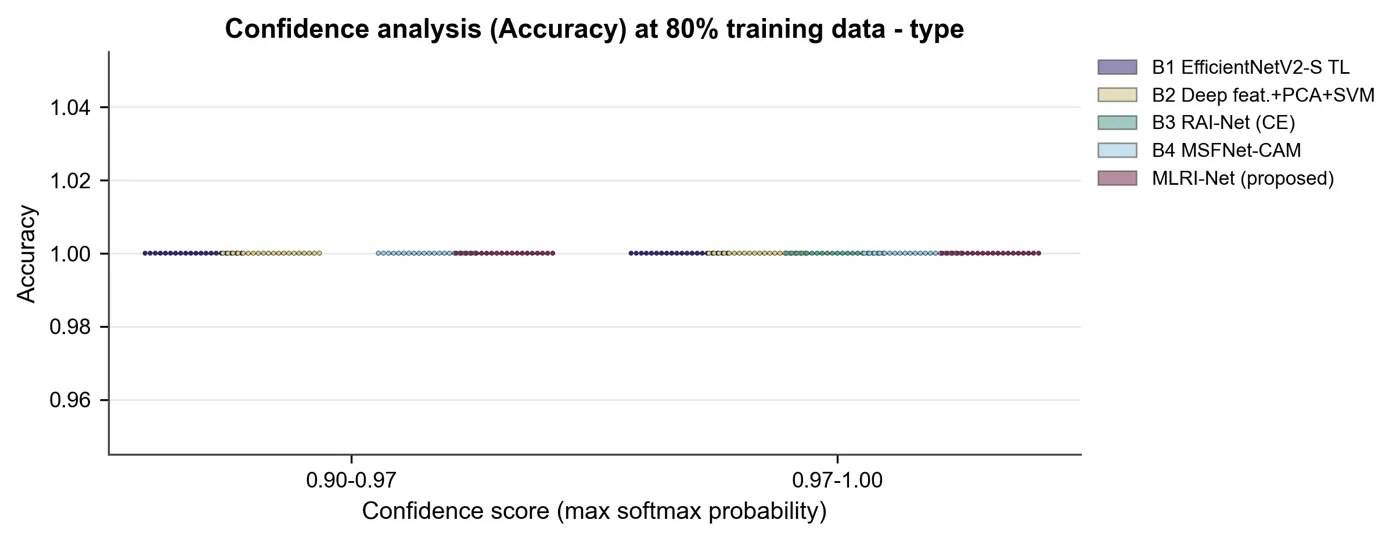
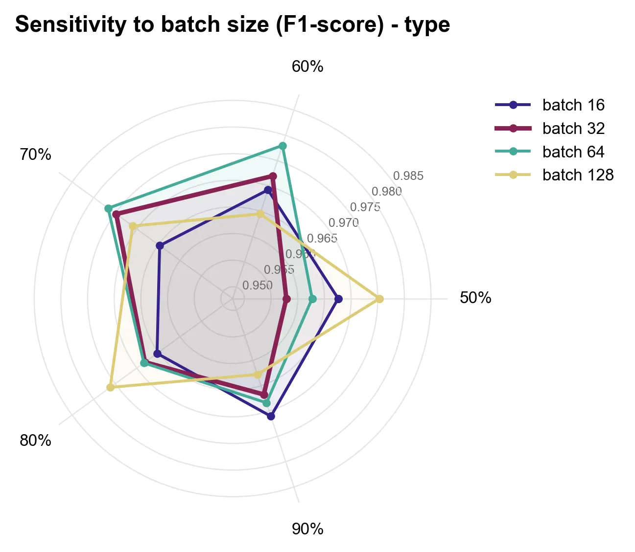
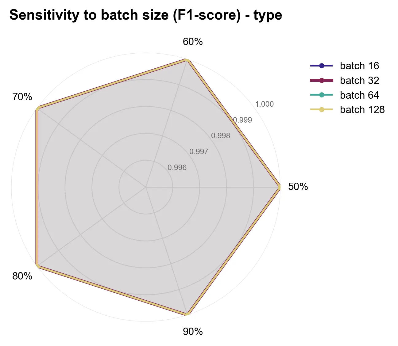
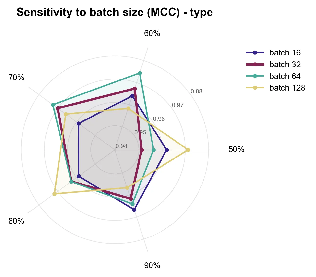
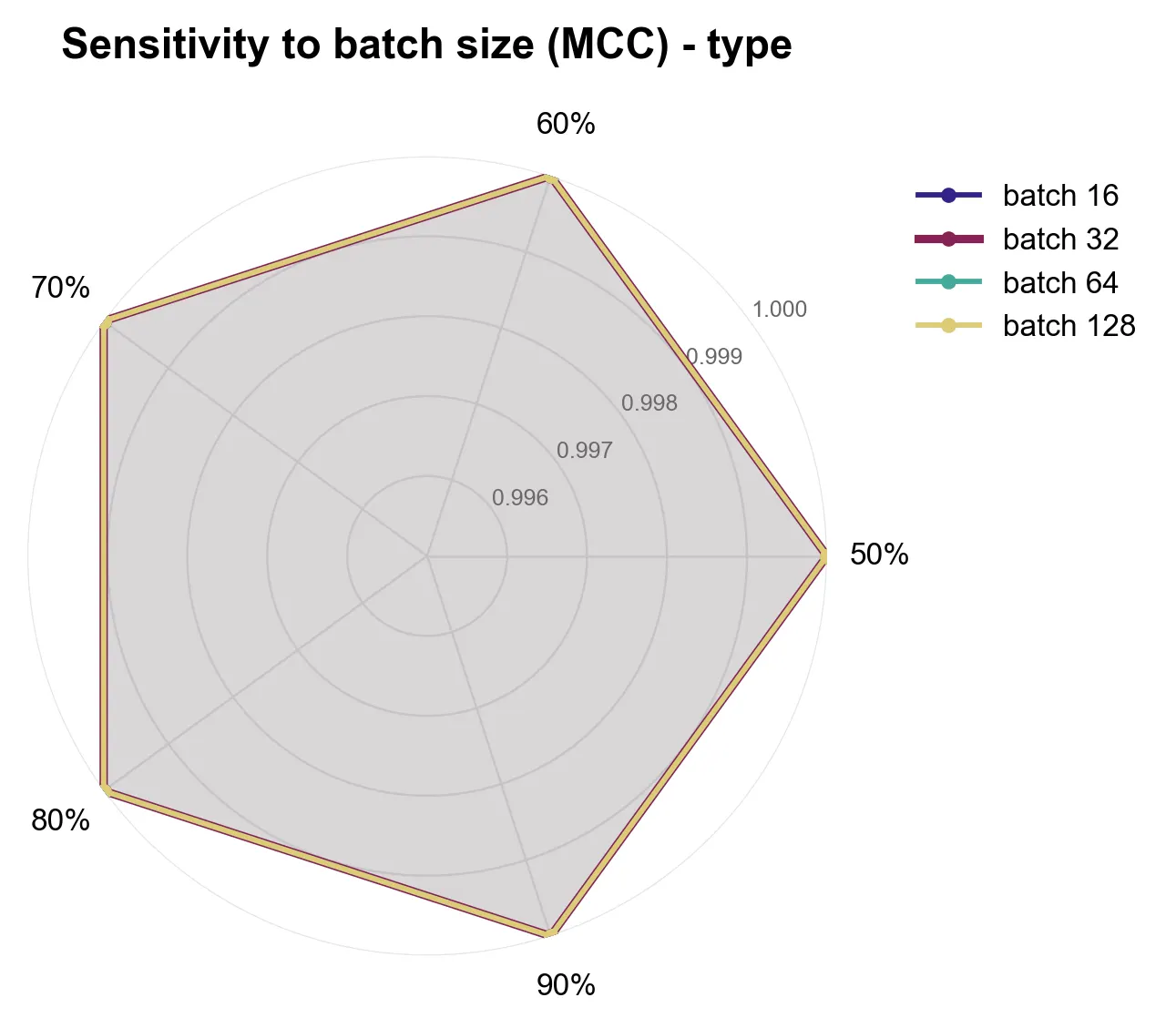
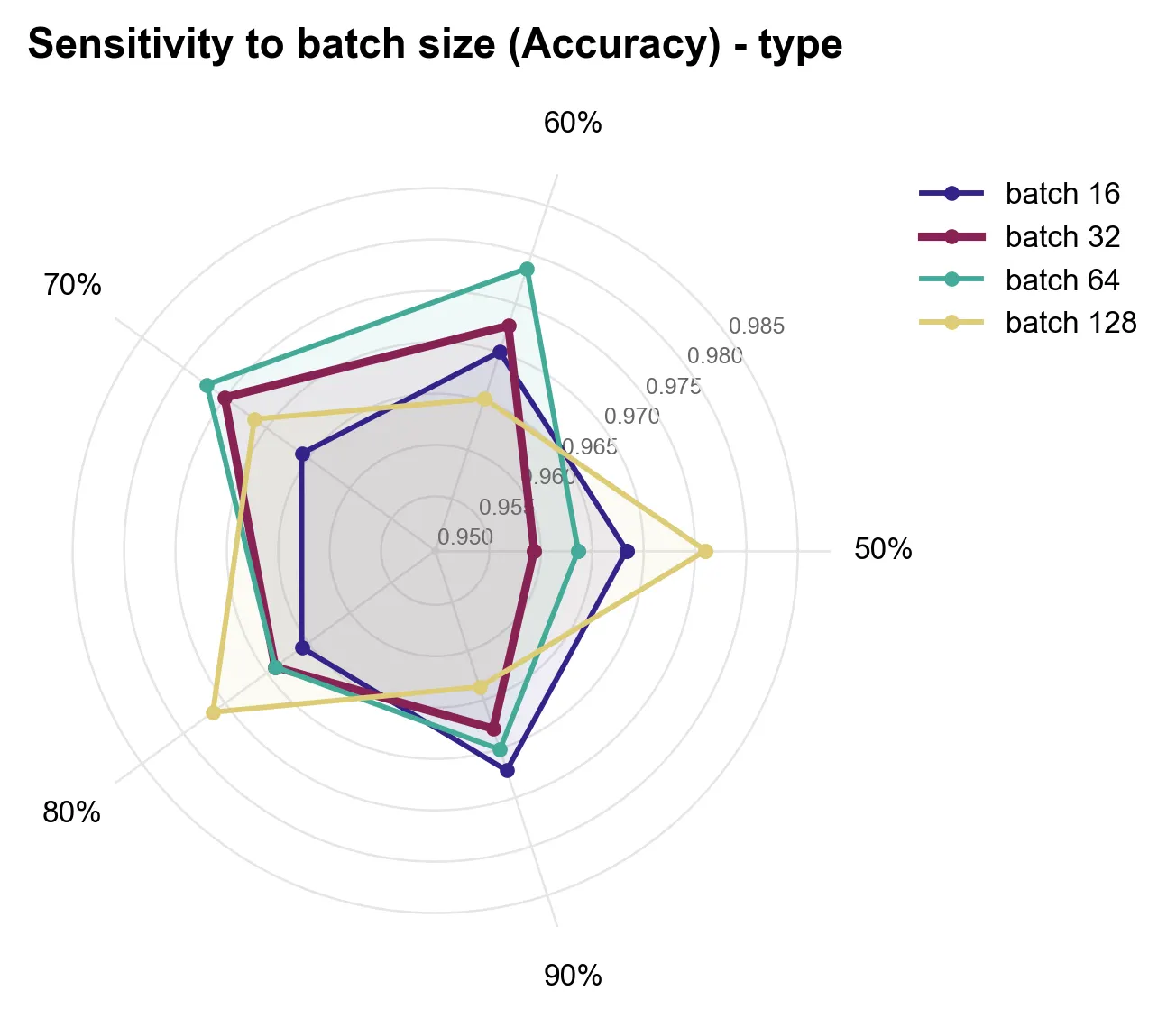
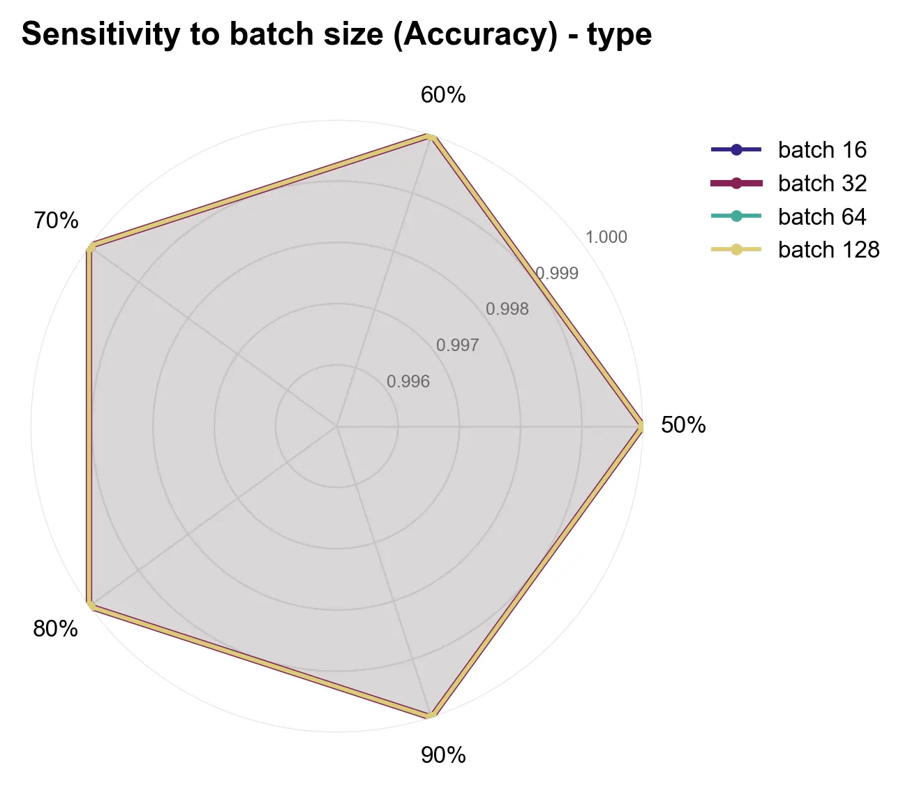
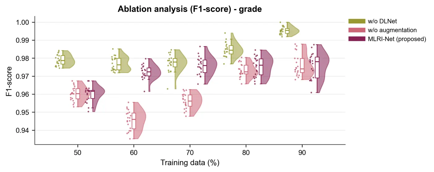
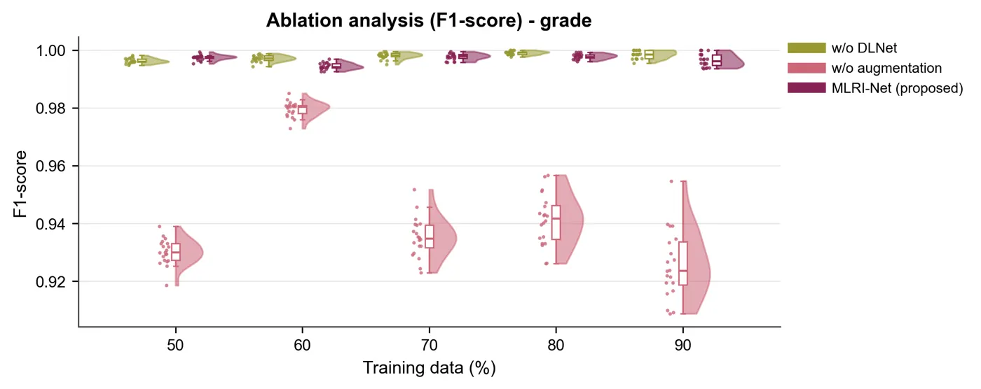
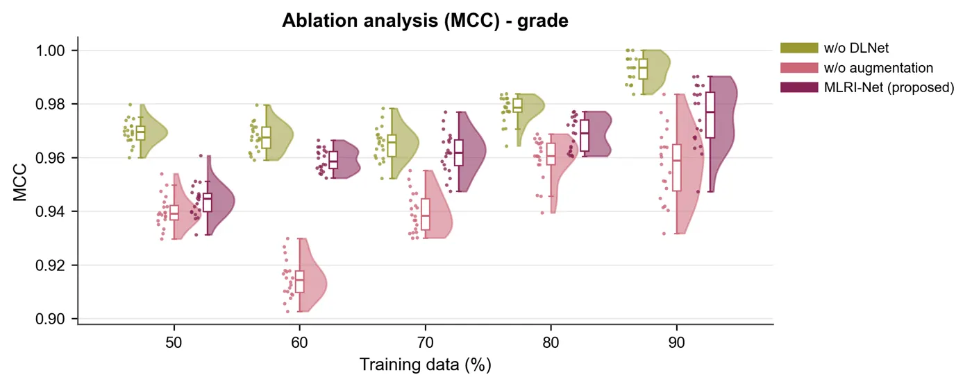
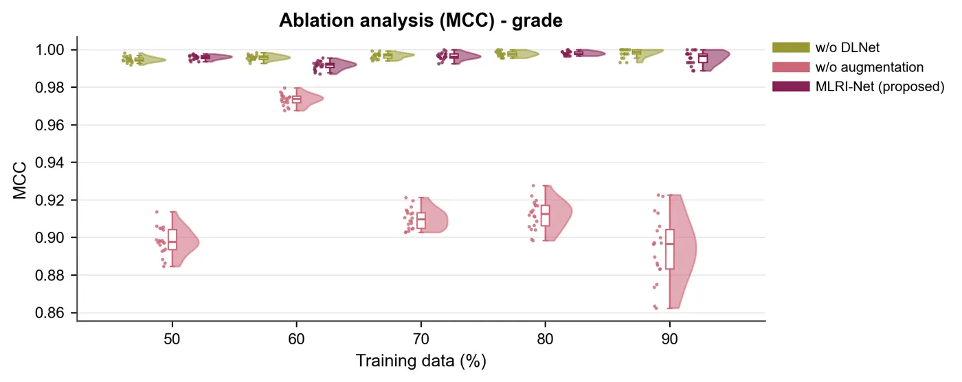
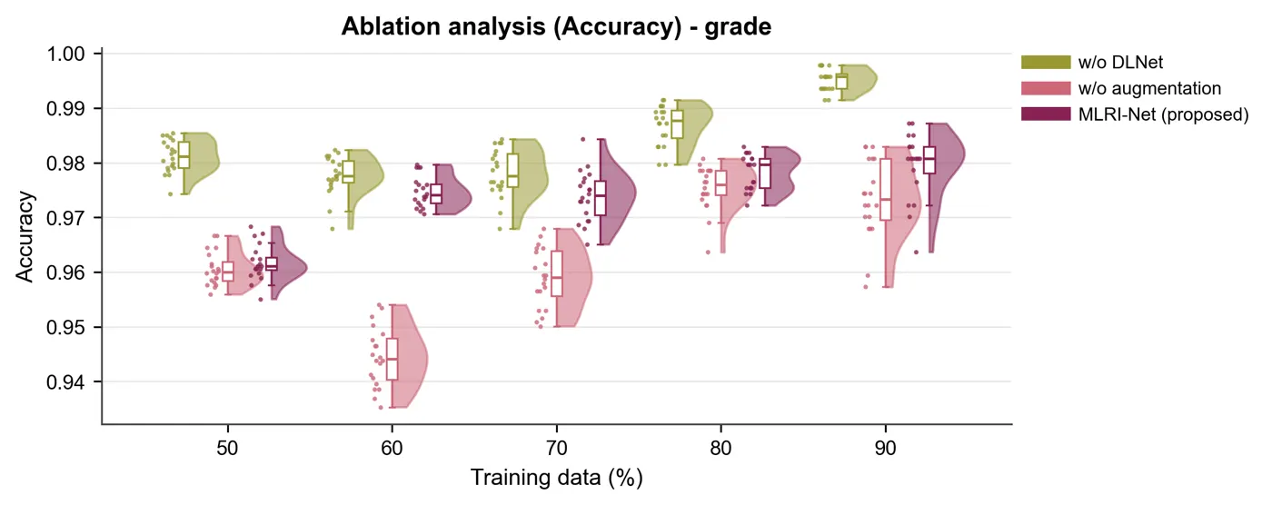
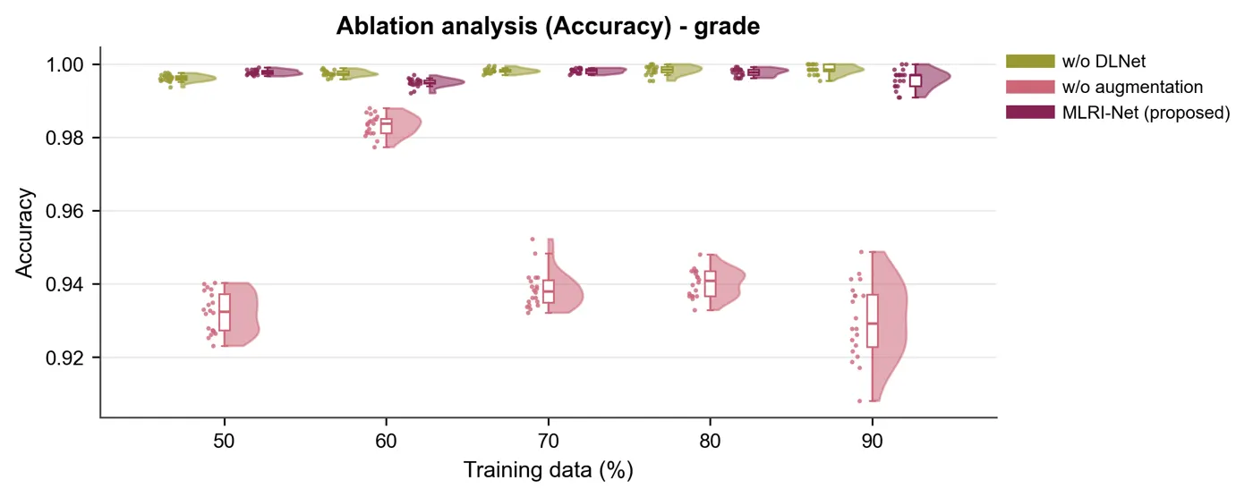
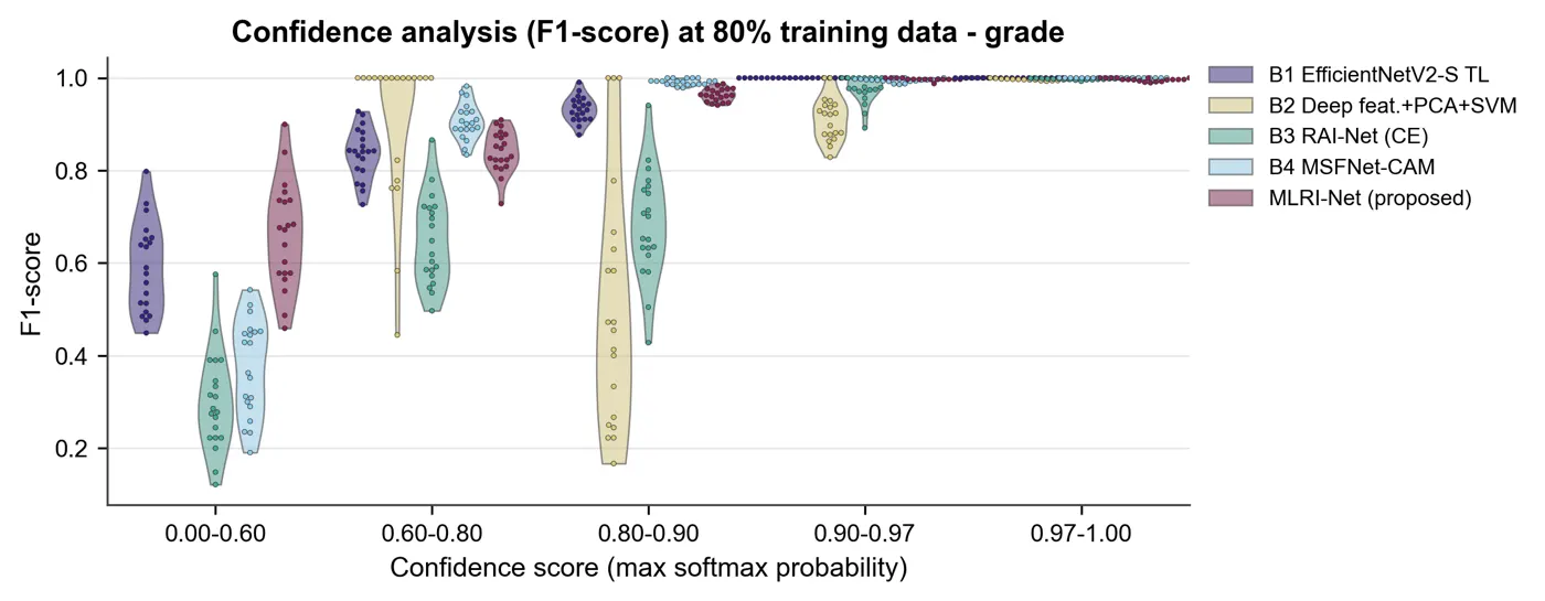
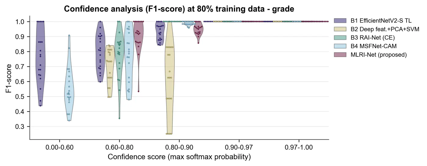
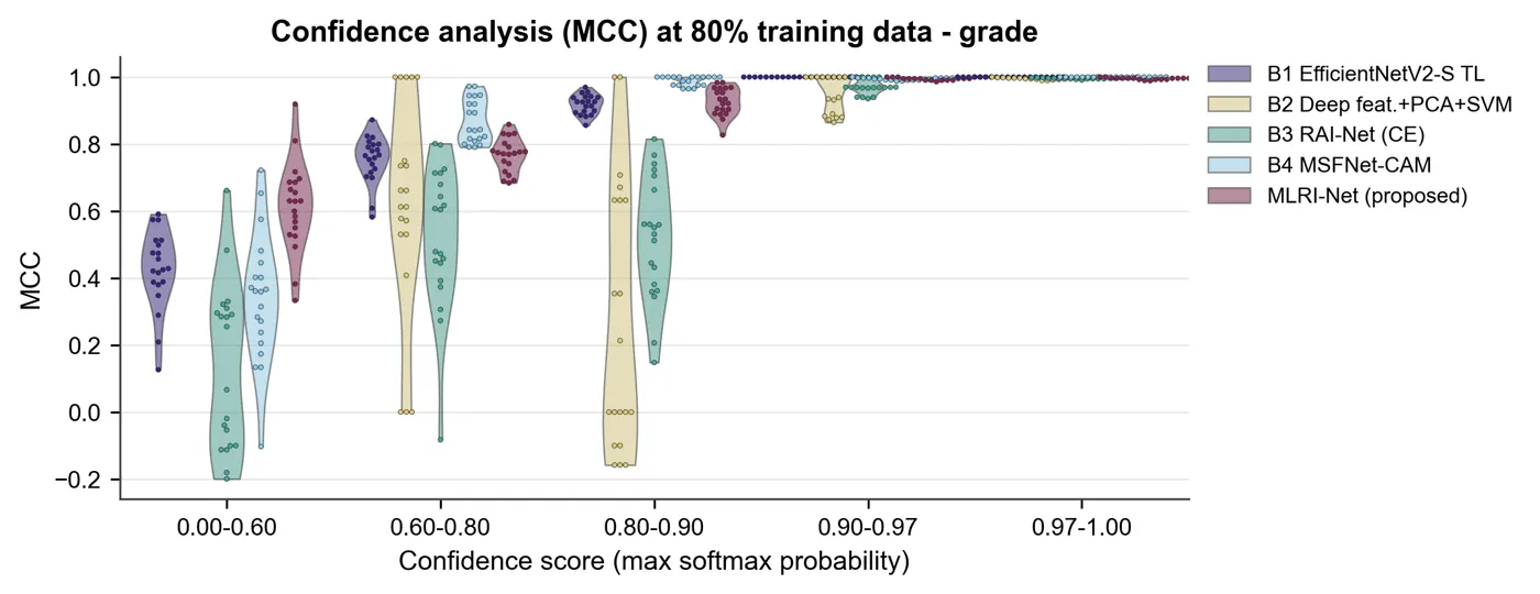
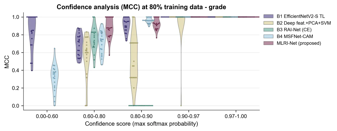
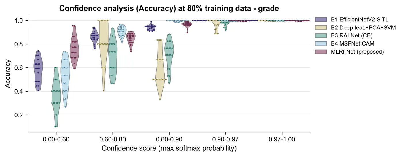
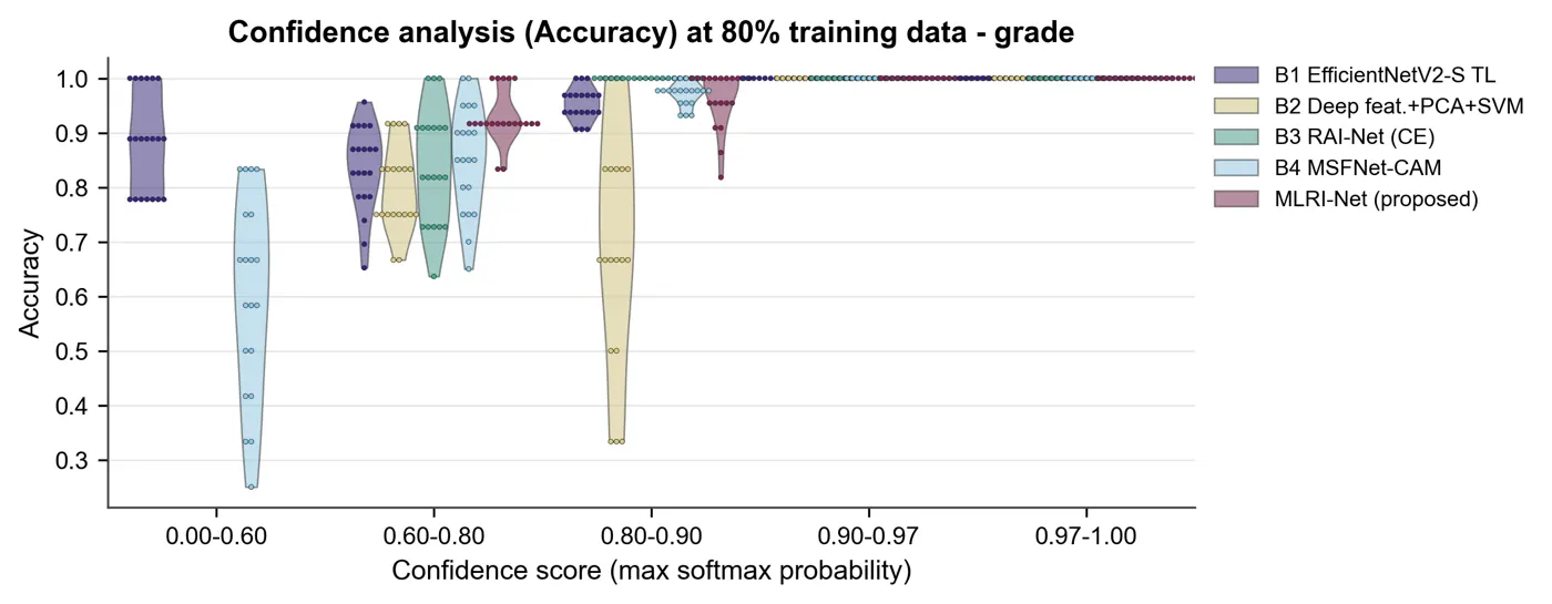
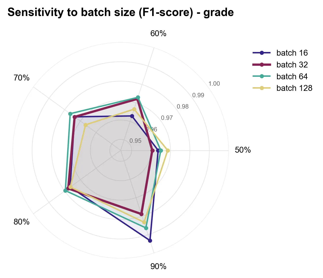
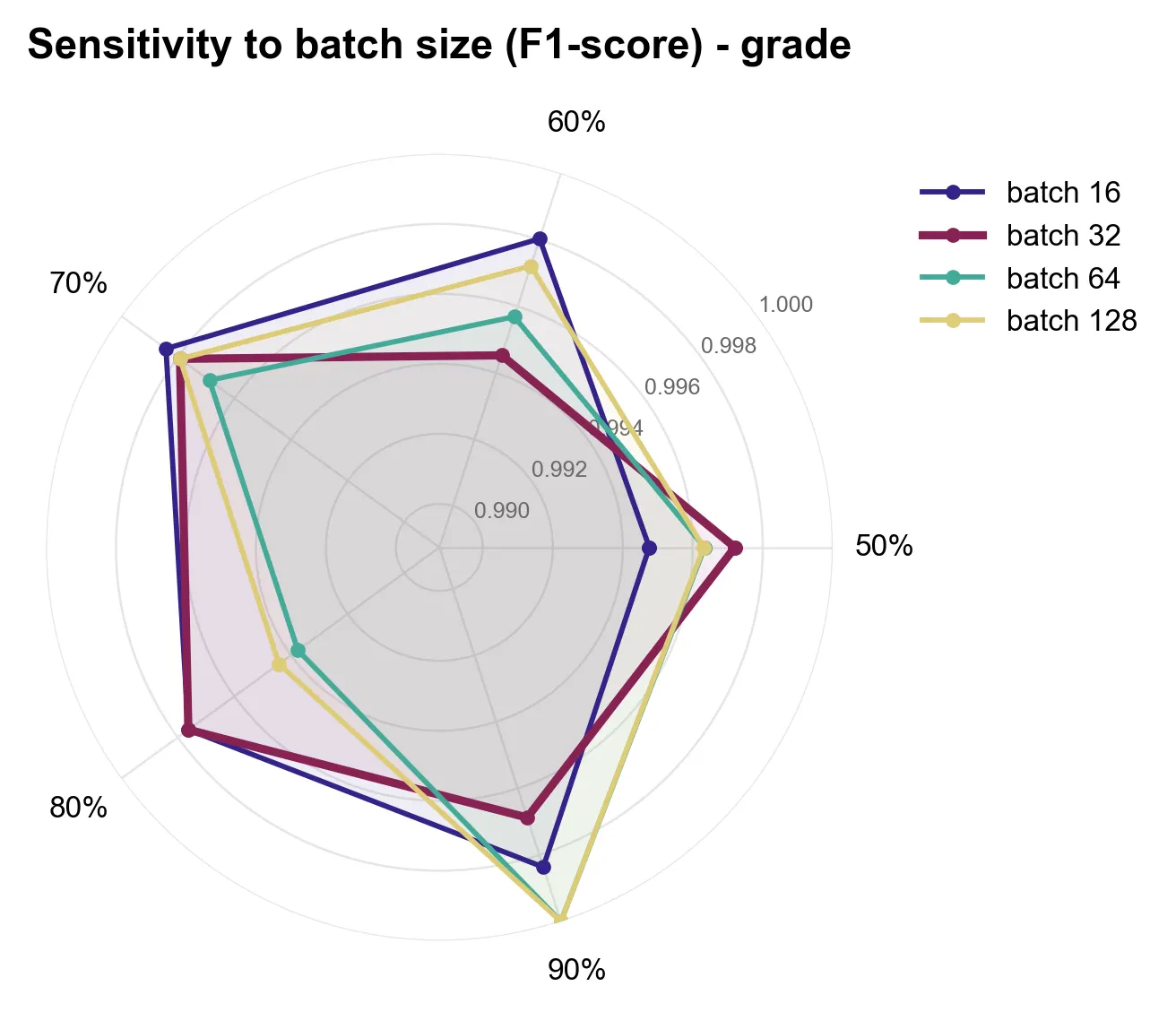
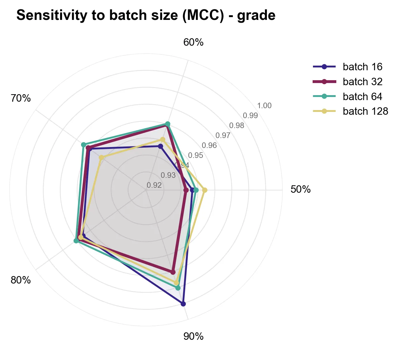
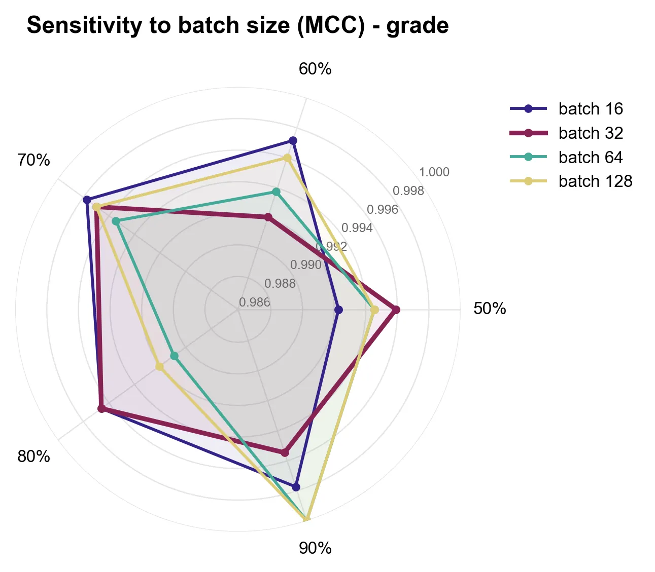
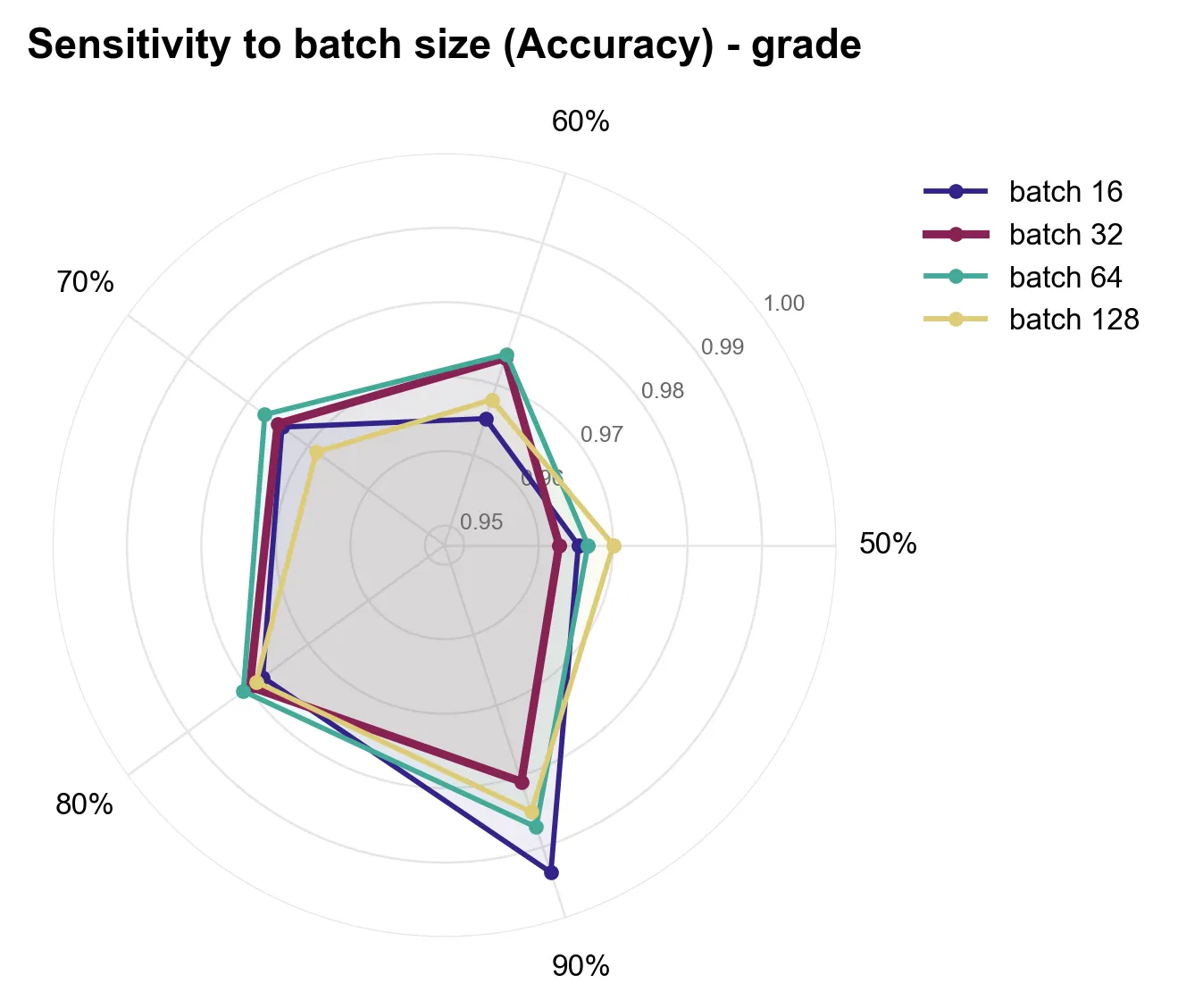
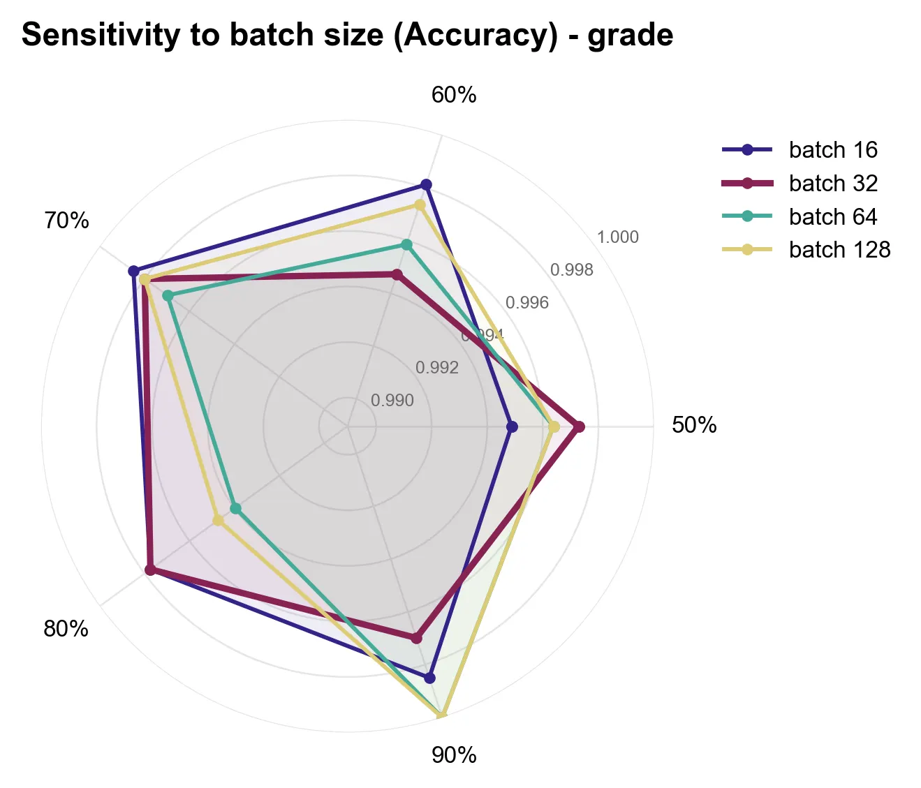
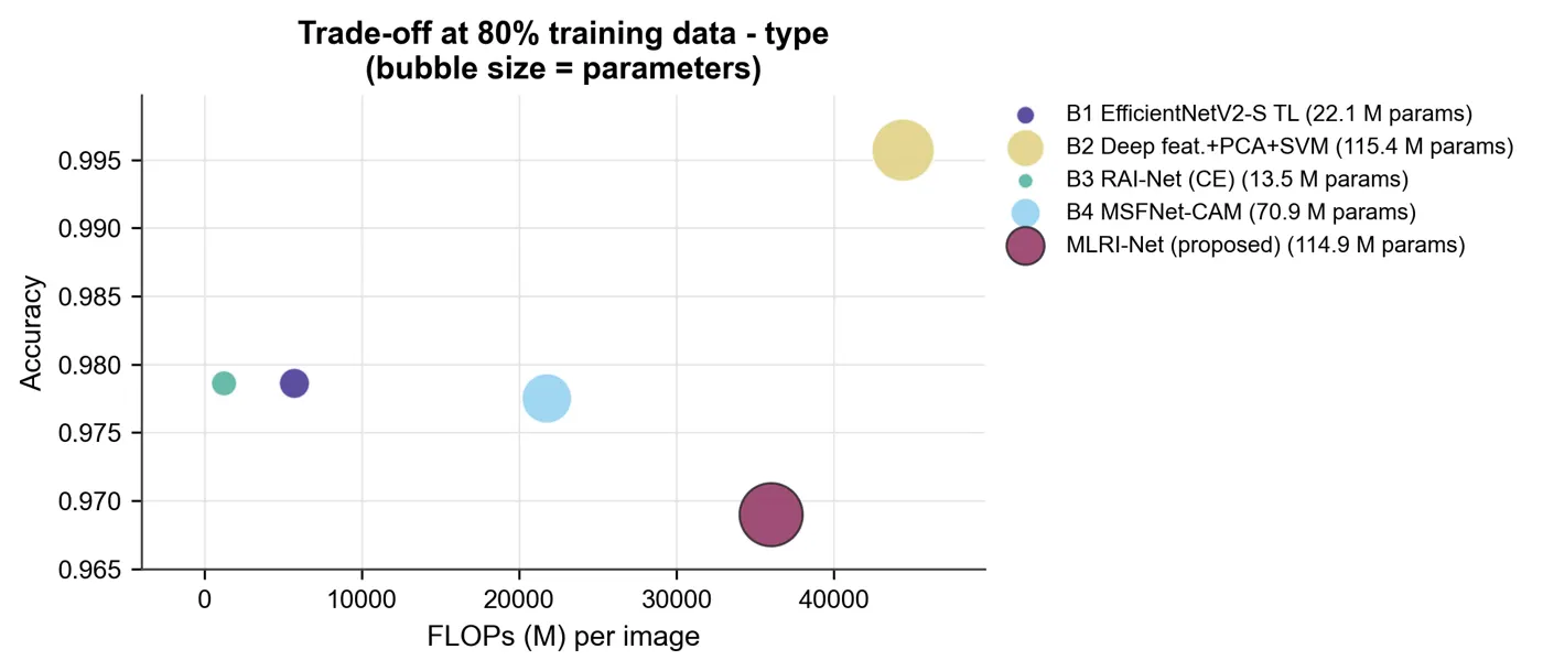
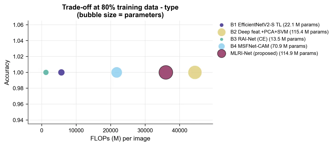
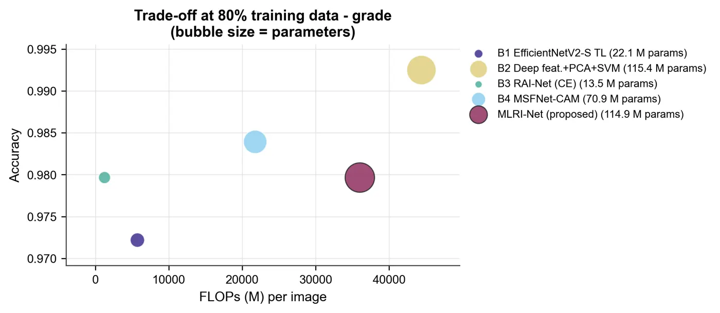
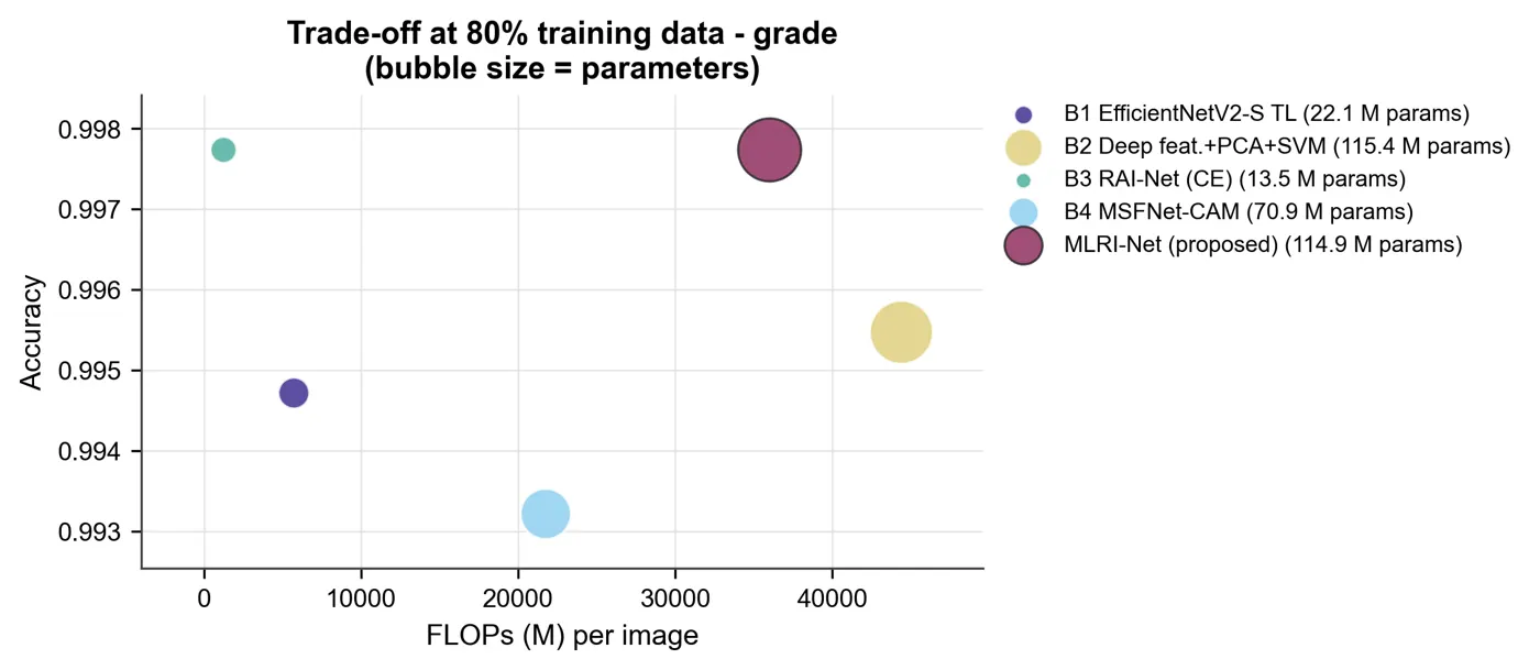
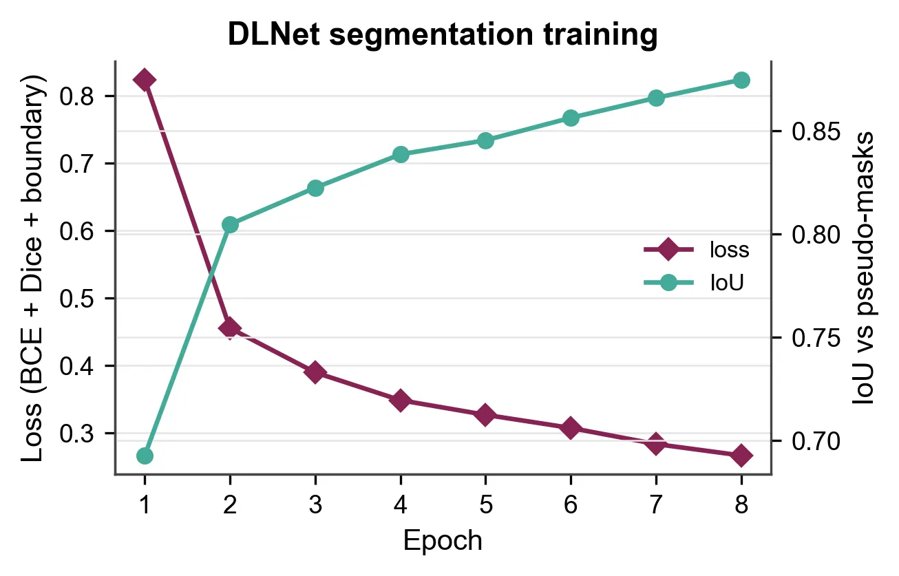
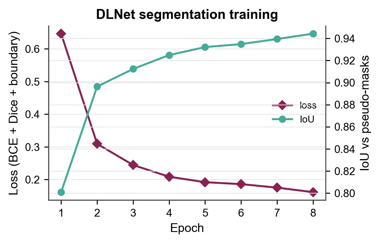
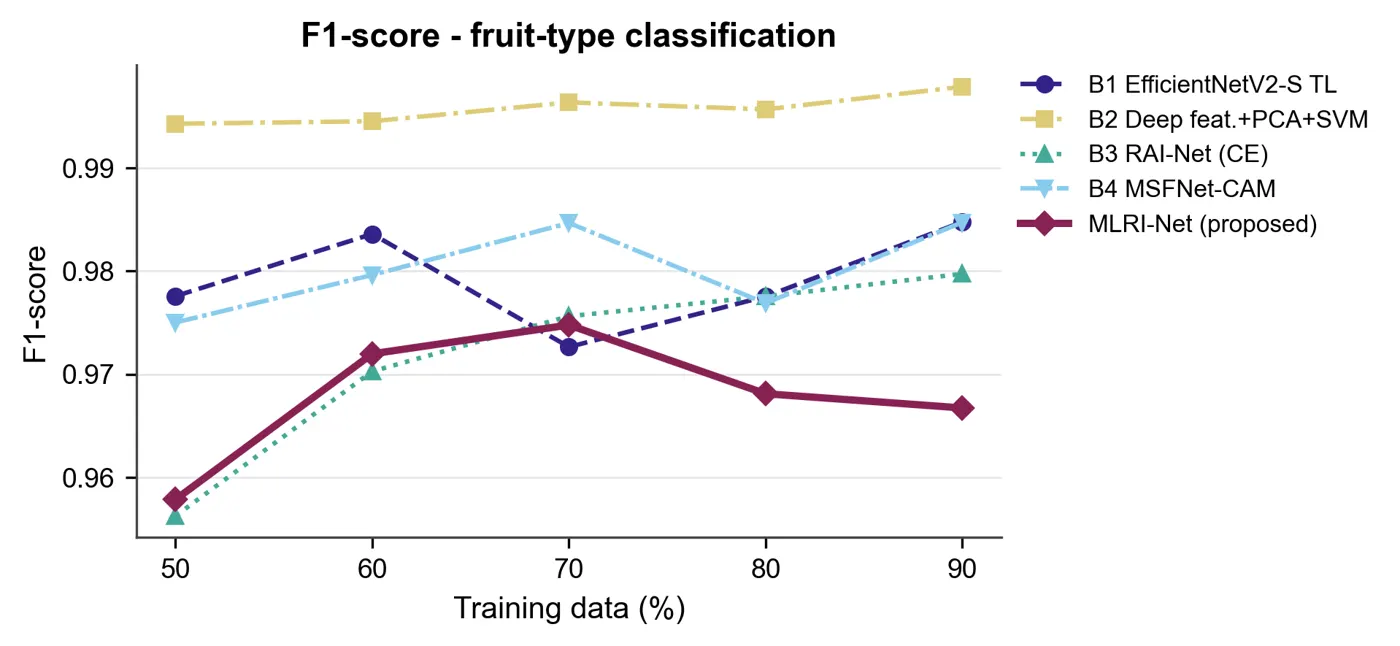
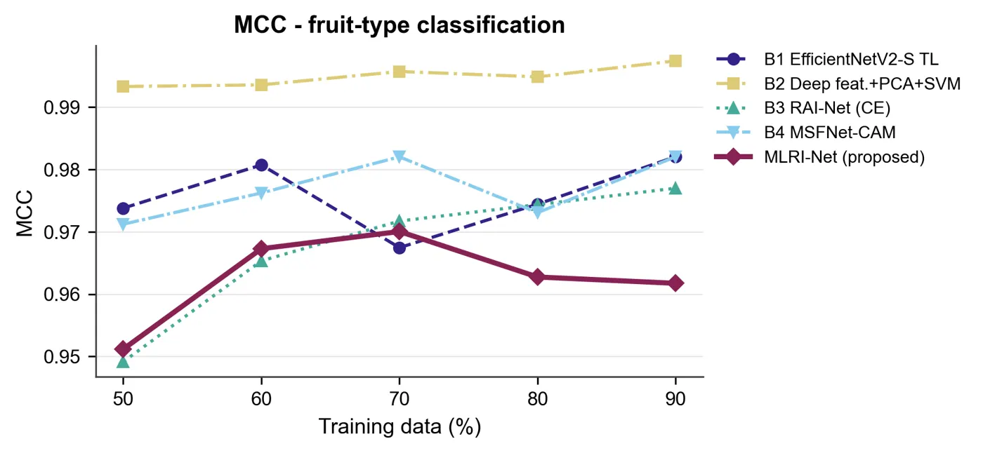
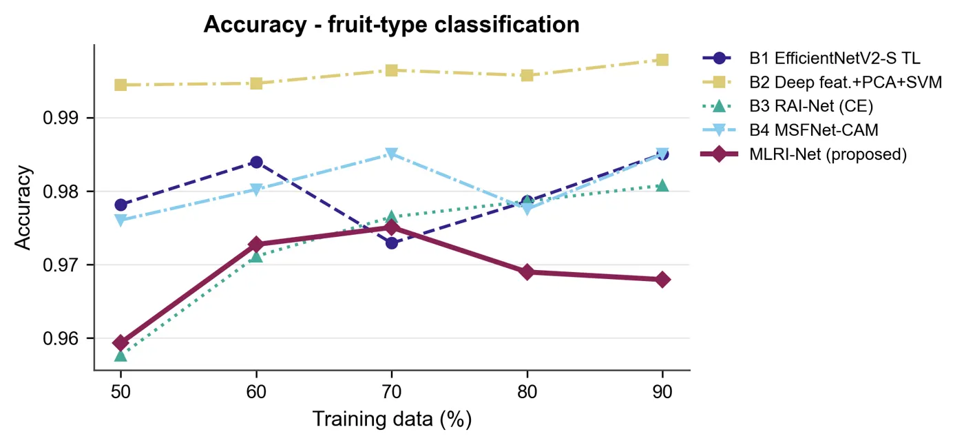
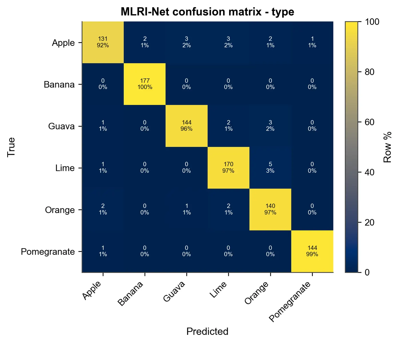
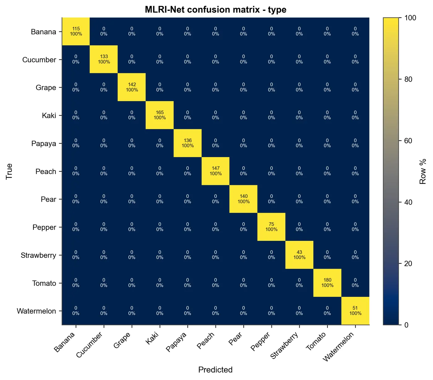
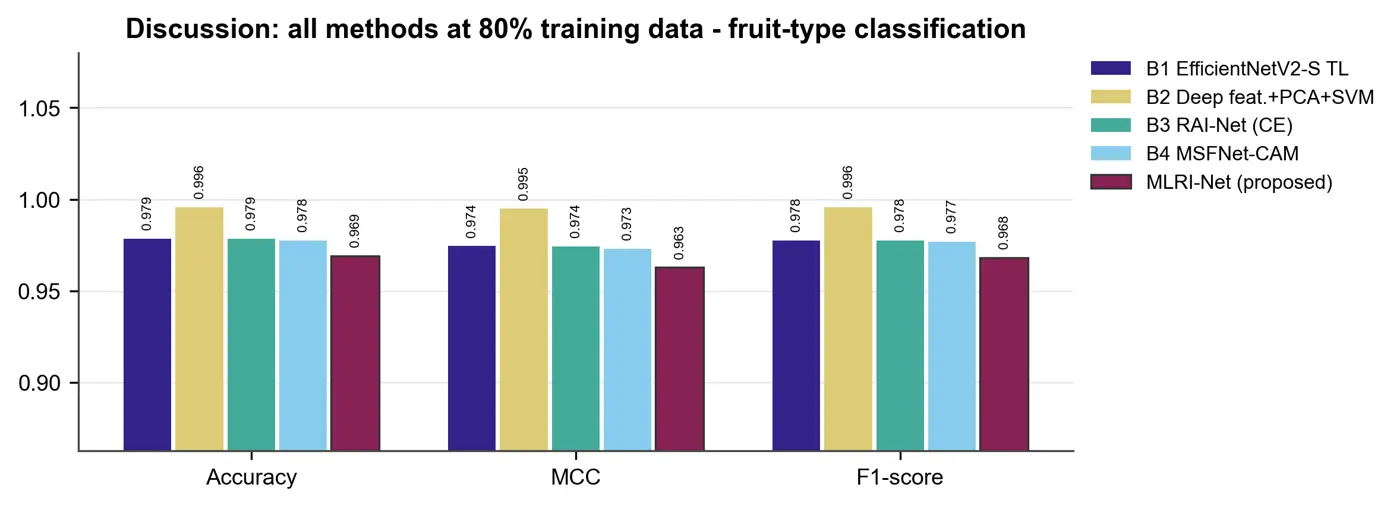
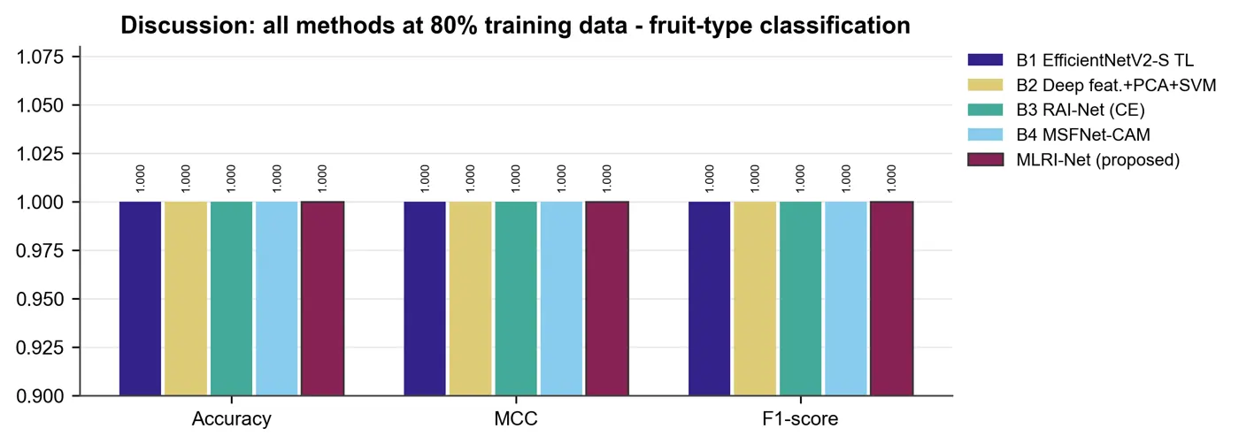
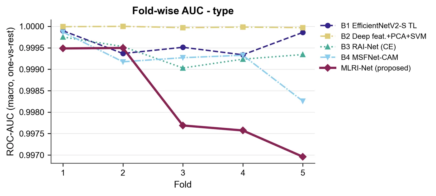
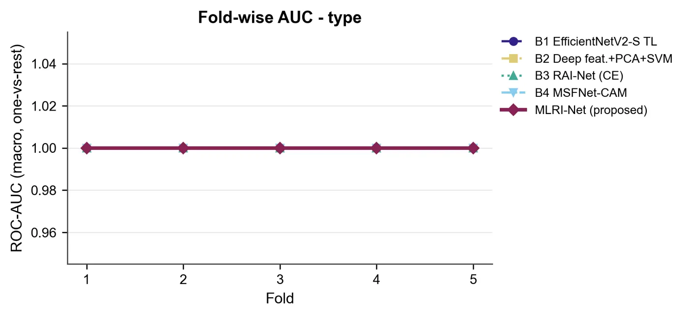
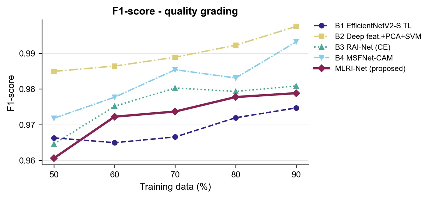
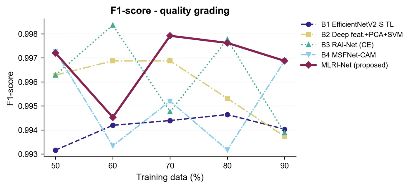
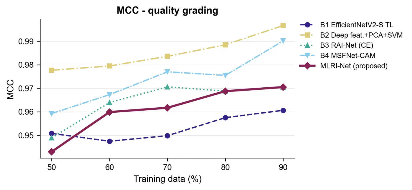
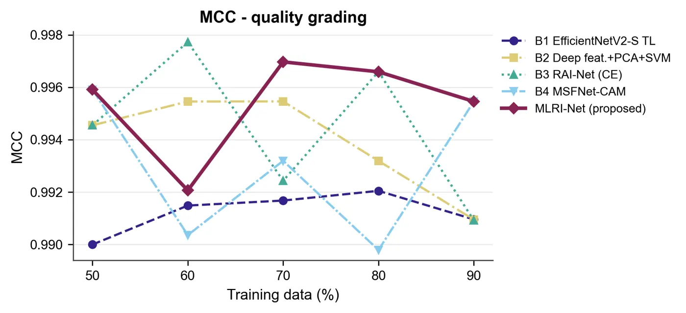
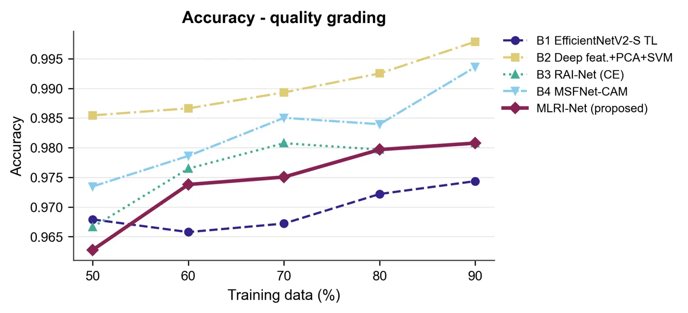
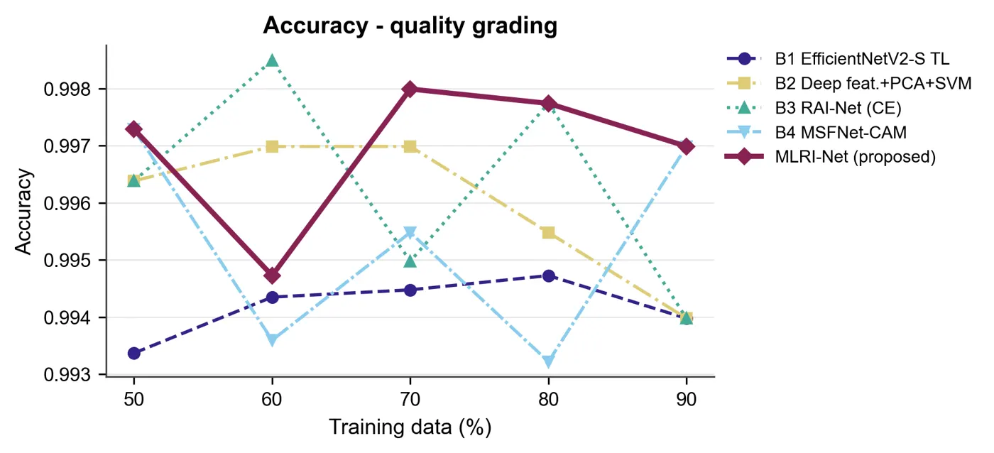
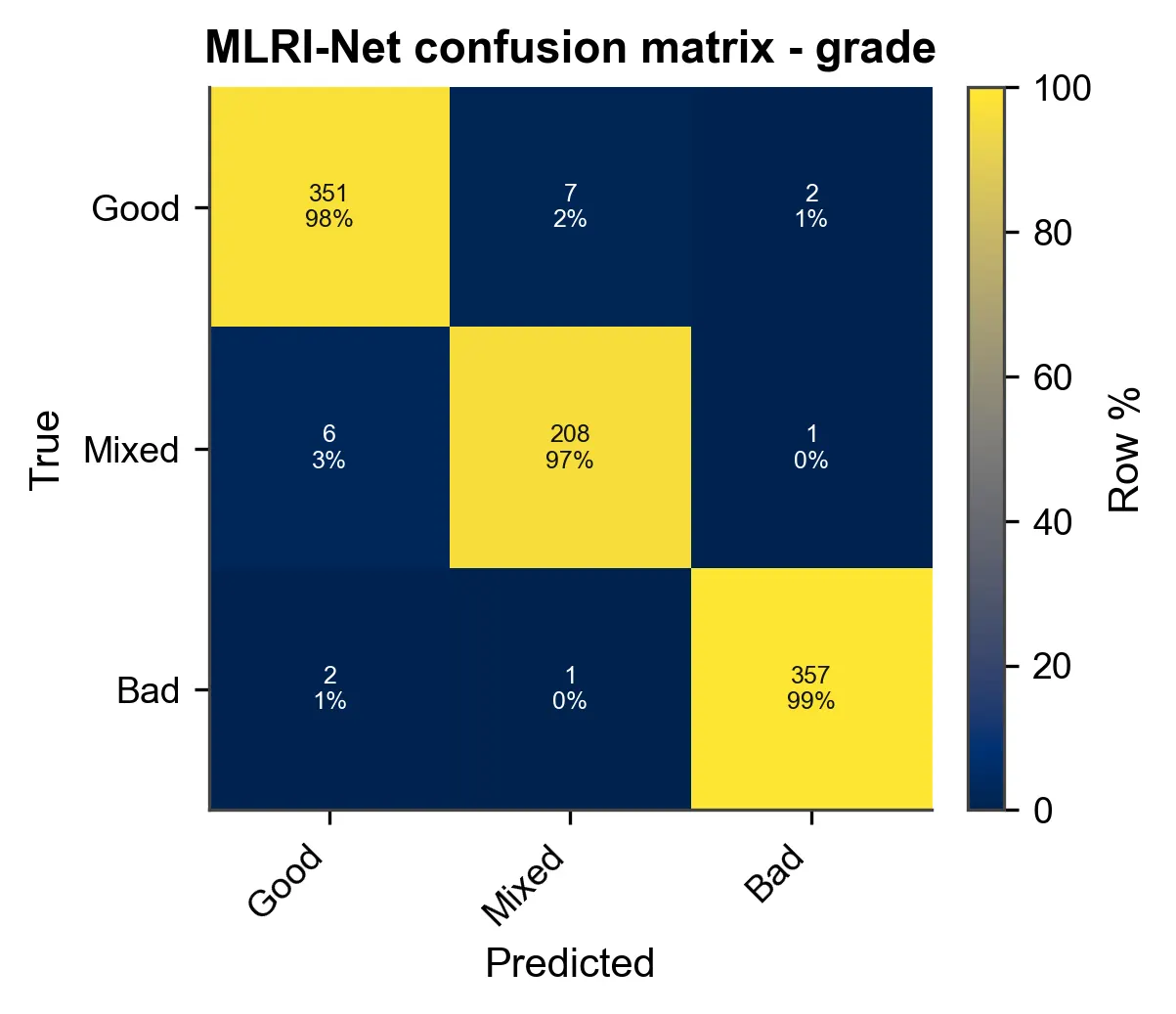
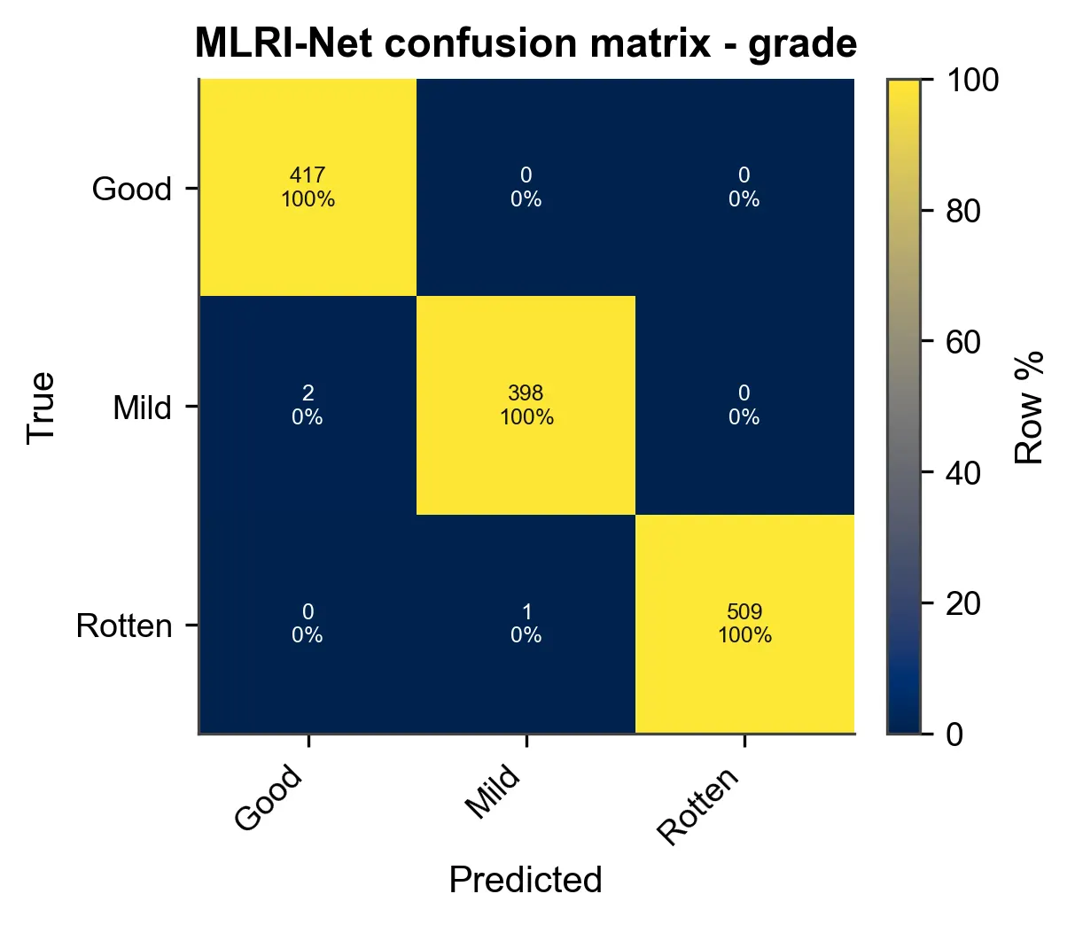
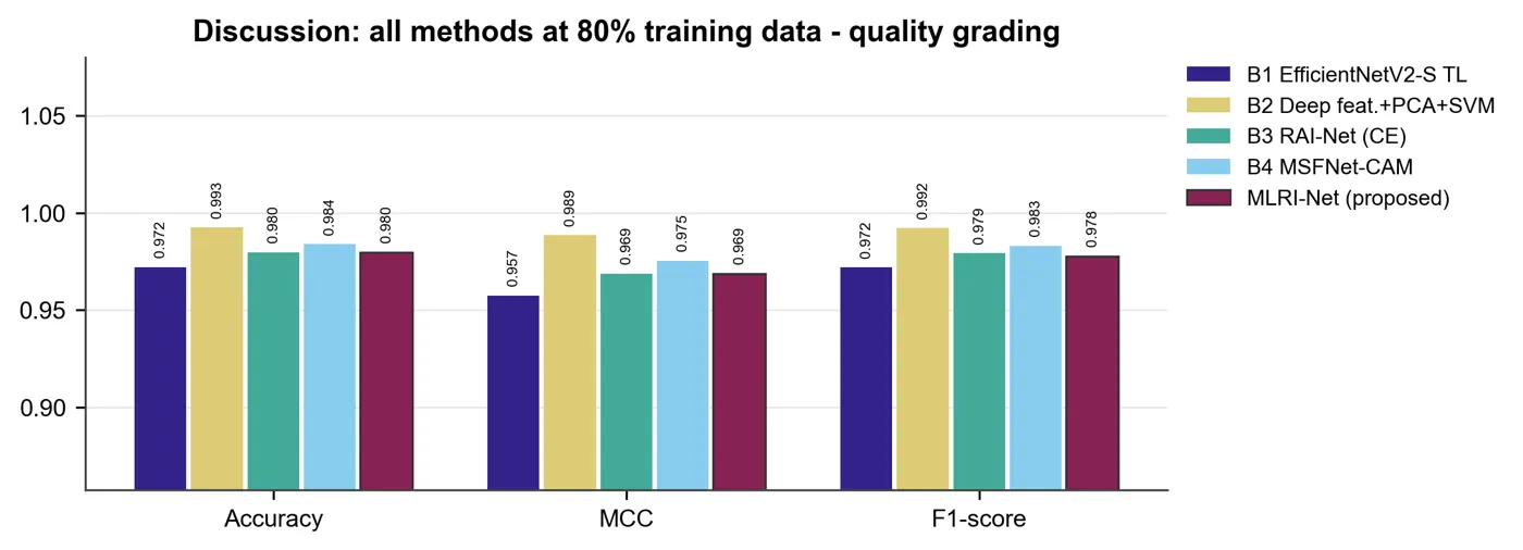
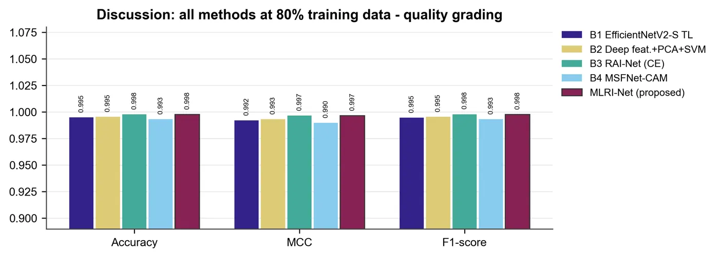
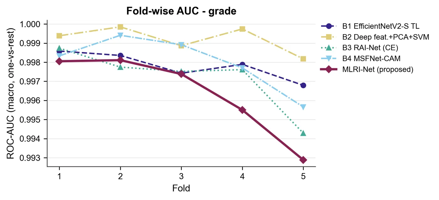
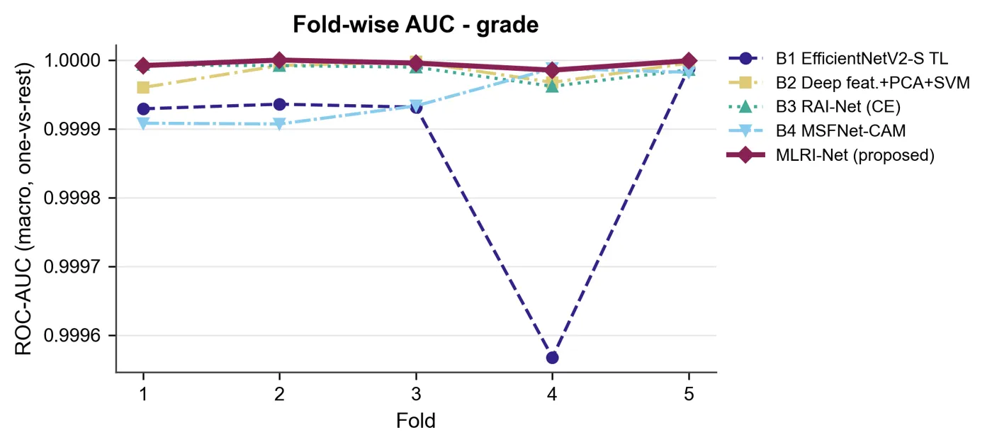
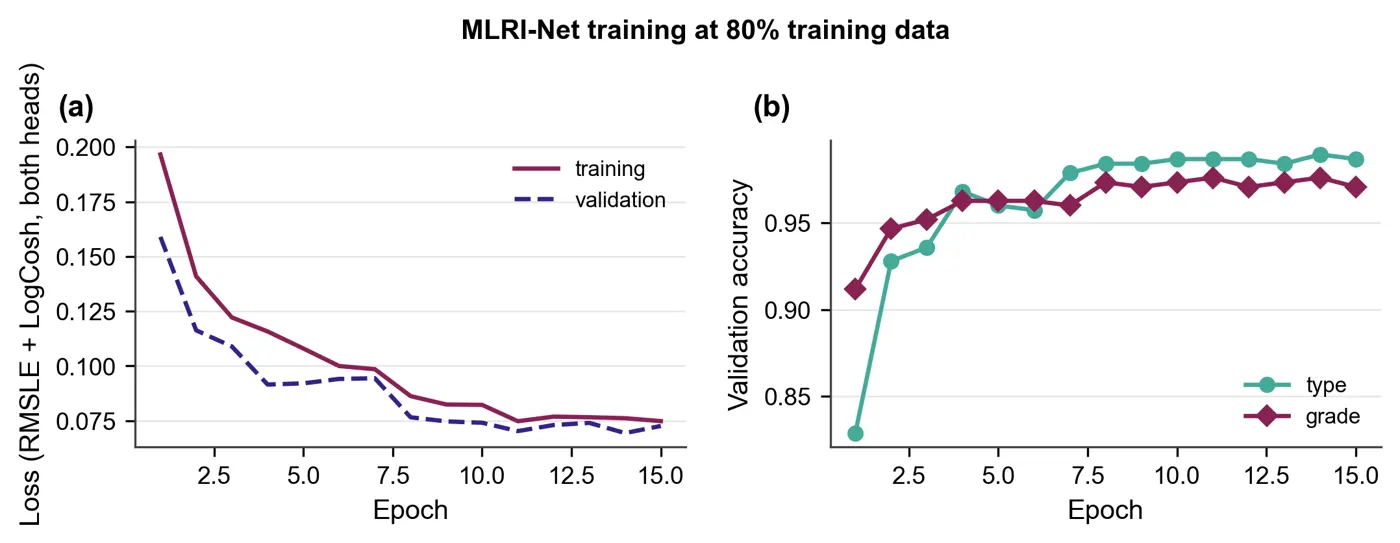
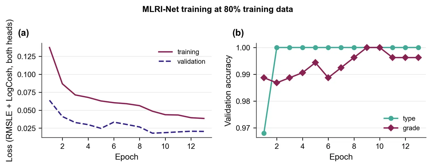
运行产生的每一张图表和示意图,按用途分组。可按组筛选,点击图表放大。
- 交付
- 85 张图表和示意图,全部展示
- 格式
- 每张图提供 PNG、矢量 PDF 和 CSV
正在加载 PDF… 0%
尚未做期刊排版的论文稿件,在 PDF 阅读器中查看,可跳页、缩放。
- 篇幅
- 31 页,排版前
- 阅读器
- 缩放、跳页、全屏、下载
正在加载 PDF… 0%
最终论文:同一份稿件按 IEEE 双栏版式排版,图表就位,参考文献已格式化。
- 最终论文
- 18 页,IEEE 双栏
- Word(DOCX)
- LaTeX 源文件
示例中的作者姓名均为占位符。
正在加载 PDF… 0%
一切从构想文档开始,连同方案、参考论文和数据集放在同一个项目文件夹里。写任何内容之前,每一项都会先被读取并评分。
- 构想 PDF,11 页手写
- Cleveland 心脏病数据集
- 参考论文
构想文档是起点。在阅读器中可以翻看全部 11 页。
"""
ShPCN-Net research control panel (tkinter GUI).

* "Run Full Pipeline & Show Graphs" runs every step for the chosen dataset(s) on a
  background thread and then shows all result graphs in the built-in viewer.
* Every pipeline step can also be run on its own from the left-hand menu.
* Settings: dataset selector (or "All datasets"), DATA_PERCENT (1-100), a toggle that
  draws a new random seed (a new set of results), and a quick smoke-test mode.

Run:  python main.py
"""
import os
import platform
import queue
import subprocess
import sys
import threading
import tkinter as tk
import traceback
from tkinter import messagebox, ttk

from PIL import Image, ImageTk

import full_pipeline_runner as runner
import run_config as cfg
from data_loader import discover_datasets

ALL_DATASETS = "All datasets"
ACCENT = "#D55E00"
INK = "#1B1B1B"
PANEL = "#F6F4F1"


def open_folder(path):
    path.mkdir(parents=True, exist_ok=True)
    if platform.system() == "Windows":
        os.startfile(str(path))
    elif platform.system() == "Darwin":
        subprocess.Popen(["open", str(path)])
    else:
        subprocess.Popen(["xdg-open", str(path)])


class ControlPanel(tk.Tk):
    def __init__(self):
        super().__init__()
        self.title("ShPCN-Net · Heart Disease Detection · Research Control Panel")
        # fit the window to the screen (laptops with 125-150 % scaling report ~1536 x 864)
        width = min(1360, self.winfo_screenwidth() - 40)
        height = min(860, self.winfo_screenheight() - 90)
        self.geometry(f"{width}x{height}+10+10")
        self.minsize(min(1000, width), min(600, height))
        self.configure(bg=PANEL)
        self.messages = queue.Queue()
        self.worker = None
        self.graph_paths = []
        self.preview_image = None
        self.datasets = list(discover_datasets())
        self._build_style()
        self._build_header()
        self._build_body()
        self._drain_job = self.after(150, self._drain_messages)
        self.refresh_gallery()
        if not self.datasets:
            messagebox.showerror("No dataset", "No non-empty code/dataset_*/ folder was found.\n"
                                               "Add the dataset before running the pipeline.")

    # ------------------------------------------------------------------ layout
    def _build_style(self):
        style = ttk.Style(self)
…
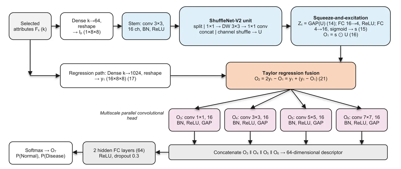
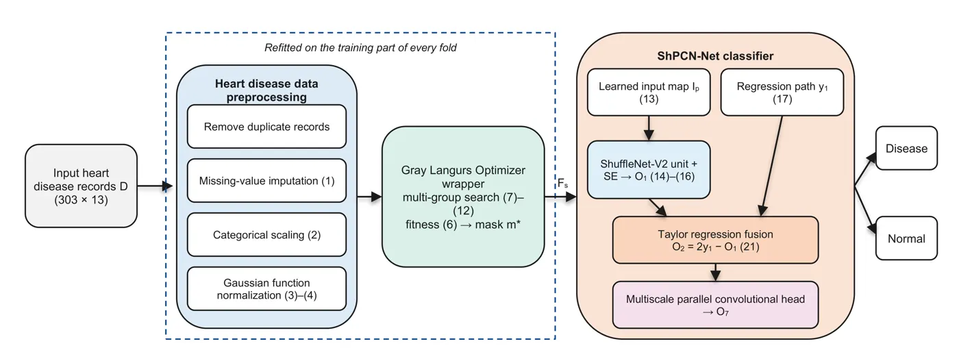
"""
Proposed method - ShPCN-Net (context.docx, Stage 3; concept handwritten diagram p.3):
F_s --(3a embedding)--> I_p --[ShuffleNet-V2 + SE]--> O1
F_s --(regression y1)--+
+--[Taylor fusion O2 = 2*y1 - O1]--> O2 --[PCNN 1/3/5/7]--> O3..O6
O7 = softmax( fc( O3 || O4 || O5 || O6 ) ) -> Disease / Normal
"""
import torch
from torch import nn
from network_building_blocks import (FeatureToMapEmbedding, HiddenDenseStack, ParallelMultiscaleConv,
ShuffleNetSEBranch, TaylorRegressionFusion)
from torch_training_loop import TorchTabularClassifier
class ShPCNNetModule(nn.Module):
def __init__(self, n_features, s):
super().__init__()
c, m = s["channels"], s["map_size"]
self.embedding = FeatureToMapEmbedding(n_features, m) # 3a
self.shufflenet_branch = ShuffleNetSEBranch(c, s["se_reduction"]) # 3b
self.taylor_fusion = TaylorRegressionFusion(n_features, c, m) # 3c
self.pcnn = ParallelMultiscaleConv(c, s["pcnn_filters"], s["pcnn_kernel_sizes"]) # 3d
self.head = HiddenDenseStack(s["pcnn_filters"] * len(s["pcnn_kernel_sizes"]),
s["hidden_neurons"], s["hidden_layers"], s["dropout_rate"],
s["activation"])
def forward(self, features, return_intermediates=False):
i_p = self.embedding(features)
o1, se_weights, unit_map = self.shufflenet_branch(i_p)
o2, y1 = self.taylor_fusion(features, o1)
pooled, branch_maps = self.pcnn(o2)
logits = self.head(pooled)
if not return_intermediates:
return logits
return logits, {
"I_p": i_p, "shufflenet_unit_map": unit_map, "se_weights": se_weights,
"O1": o1, "y1": y1, "O2": o2,
"O3": branch_maps[0], "O4": branch_maps[1], "O5": branch_maps[2], "O6": branch_maps[3],
"O7": torch.softmax(logits, dim=1),
}
class ShPCNNetClassifier(TorchTabularClassifier):
display_name = "ShPCN-Net (proposed)"
def build_module(self, n_features):
return ShPCNNetModule(n_features, self.settings)
def trace_intermediates(self, X):
"""Every intermediate tensor (as numpy) for visualisation of one or more samples."""
self.module.eval()
with torch.no_grad():
_, inter = self.module(torch.as_tensor(X, dtype=torch.float32), return_intermediates=True)
return {k: v.numpy() for k, v in inter.items()}
"""
Stage 2 - feature selection with the Gray Langurs Optimizer (GLO)  (N_d -> F_s).

Source: Barshandeh et al., "Gray langurs optimizer: a multi-group bio-inspired
optimization algorithm" (Artificial Intelligence Review, 2026). The paper is not
in basepapers/, so the equations below follow its published description (three
group types: one-male, multi-male and all-male groups; social hierarchy;
migration between groups after alpha death / mate finding / puberty; arbitrary
movement inside the territory). The exact coefficients are our documented
interpretation - see context.docx "Open questions".

Notation (per langur i, dimension d, iteration t of T):
  a      = a_start - (a_start - a_end) * t / (T - 1)       control parameter, 2 -> 0
  r1,r2,r3 ~ U(0,1)
  One-male group  (follow the single alpha A_g):
      X_new = A_g - a * (2*r1 - 1) * |r2 * A_g - X_i|
  Multi-male group (follow the mean M_g of the top-3 males + global best G):
      X_new = M_g - a * (2*r1 - 1) * |r2 * M_g - X_i| + r3 * (1 - a/a_start) * (G - X_i)
  All-male group  (bachelors roam: random partner X_j + pull to G for mate finding):
      X_new = X_i + a * (2*r1 - 1) * (X_j - X_i) + r2 * (1 - a/a_start) * (G - X_i)
  Territory movement (probability p_rand):
      X_new = X_i + a * N(0, 0.1 * (ub - lb))
  Greedy replacement: X_i <- X_new only if fitness improves.
  Alpha death: if a group's best fitness has not improved for L iterations, its
      worst member is re-born near the global best (puberty / new male joins).
  Migration: every M iterations the worst member of group g swaps with a random
      member of group g+1 (langurs move between groups).
  Boundaries: positions are clipped to [lb, ub].

Solution encoding (context.docx 3.3.1): position vector in [0,1]^N, feature d is
selected when X_d > 0.5 -> equivalent to the list of selected feature indices.
Fitness (Eq. 24): Fitness = alpha*(1 - Accuracy) + (1 - alpha) * R / K  (minimised),
Accuracy from an RBF-SVM wrapper with stratified inner CV on the training data only.
"""
import numpy as np
from sklearn.model_selection import StratifiedKFold, cross_val_score
from sklearn.svm import SVC

import run_config as cfg

GROUP_TYPES = ("one_male", "multi_male", "all_male")


def position_to_mask(position, threshold):
    """Continuous langur position -> boolean feature mask (at least one feature)."""
    mask = position > threshold
    if not mask.any():
        mask[int(np.argmax(position))] = True
    return mask


class FeatureSubsetFitness:
    """Eq. (24) wrapper fitness with a cache (identical masks are scored once)."""

    def __init__(self, X, y, alpha, cv_folds, svm_c, seed, threshold):
        self.X, self.y = X, y
        self.alpha, self.threshold = alpha, threshold
        n_splits = int(max(2, min(cv_folds, np.bincount(y).min())))
        self.cv = StratifiedKFold(n_splits=n_splits, shuffle=True, random_state=seed)
        self.svm_c = svm_c
        self.cache = {}

    def accuracy_of(self, mask):
        key = tuple(np.flatnonzero(mask))
        if key not in self.cache:
            model = SVC(C=self.svm_c, kernel="rbf", gamma="scale")
            self.cache[key] = float(cross_val_score(model, self.X[:, mask], self.y, cv=self.cv).mean())
        return self.cache[key]

    def __call__(self, position):
…
"""
Reusable PyTorch blocks for ShPCN-Net and the ablation baselines (context.docx, Stage 3).
FeatureToMapEmbedding 3a: k selected features -> learned 1 x 8 x 8 map I_p
ShuffleNetV2Unit 3b: channel split, 1x1 conv, 3x3 depthwise conv, 1x1 conv,
concatenation, channel shuffle
SqueezeExcitation 3b: Eq. 8-10 Z_c = 1/(H*W) sum_i sum_j I_p
s = sigma(W2 * delta(W1 * Z_c))
O1 = s * I_p
TaylorRegressionFusion 3c: y1 = sum F_i * w_i (learned map to the shape of O1)
O2 = 2*y1 - O1 (first-order Taylor rule, k = 1)
ParallelMultiscaleConv 3d: O3..O6 = f_conv1..4(O2) with 1/3/5/7 kernels
HiddenDenseStack FC hidden layers (depth = "hidden layers" setting)
"""
import torch
from torch import nn
def make_activation(name):
return {"relu": nn.ReLU(), "gelu": nn.GELU(), "elu": nn.ELU(), "tanh": nn.Tanh()}.get(name, nn.ReLU())
class FeatureToMapEmbedding(nn.Module):
"""Dense k -> map_size^2, reshaped to (B, 1, H, W). This is the network input I_p."""
def __init__(self, n_features, map_size):
super().__init__()
self.map_size = map_size
self.linear = nn.Linear(n_features, map_size * map_size)
def forward(self, x):
return self.linear(x).view(-1, 1, self.map_size, self.map_size)
def channel_shuffle(x, groups):
b, c, h, w = x.shape
return x.view(b, groups, c // groups, h, w).transpose(1, 2).contiguous().view(b, c, h, w)
class ShuffleNetV2Unit(nn.Module):
"""Stride-1 ShuffleNet-V2 basic unit (Ma et al., 2018)."""
def __init__(self, channels):
super().__init__()
half = channels // 2
self.branch = nn.Sequential(
nn.Conv2d(half, half, 1, bias=False), nn.BatchNorm2d(half), nn.ReLU(inplace=True),
nn.Conv2d(half, half, 3, padding=1, groups=half, bias=False), nn.BatchNorm2d(half),
nn.Conv2d(half, half, 1, bias=False), nn.BatchNorm2d(half), nn.ReLU(inplace=True),
)
def forward(self, x):
left, right = x.chunk(2, dim=1) # channel split
out = torch.cat([left, self.branch(right)], dim=1) # concatenation
return channel_shuffle(out, 2) # channel shuffle
class SqueezeExcitation(nn.Module):
"""Eq. 8-10. Returns (O1, s) so the attention weights can be visualised."""
def __init__(self, channels, reduction):
super().__init__()
hidden = max(channels // reduction, 2)
self.w1 = nn.Linear(channels, hidden) # W1
self.w2 = nn.Linear(hidden, channels) # W2
self.delta = nn.ReLU() # delta
self.sigma = nn.Sigmoid() # sigma
def forward(self, i_p):
z_c = i_p.mean(dim=(2, 3)) # Eq. 8: global average pooling
…EasySeer 把项目写成若干个独立的 Python 文件,外加一个主程序。可以打开任意文件阅读,也可以在对话中问它做了什么。
- 项目内容
- 47 个 Python 文件,另有 requirements 和 readme
- 展示
- 四个真实文件的开头几行
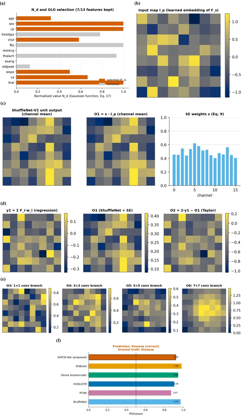
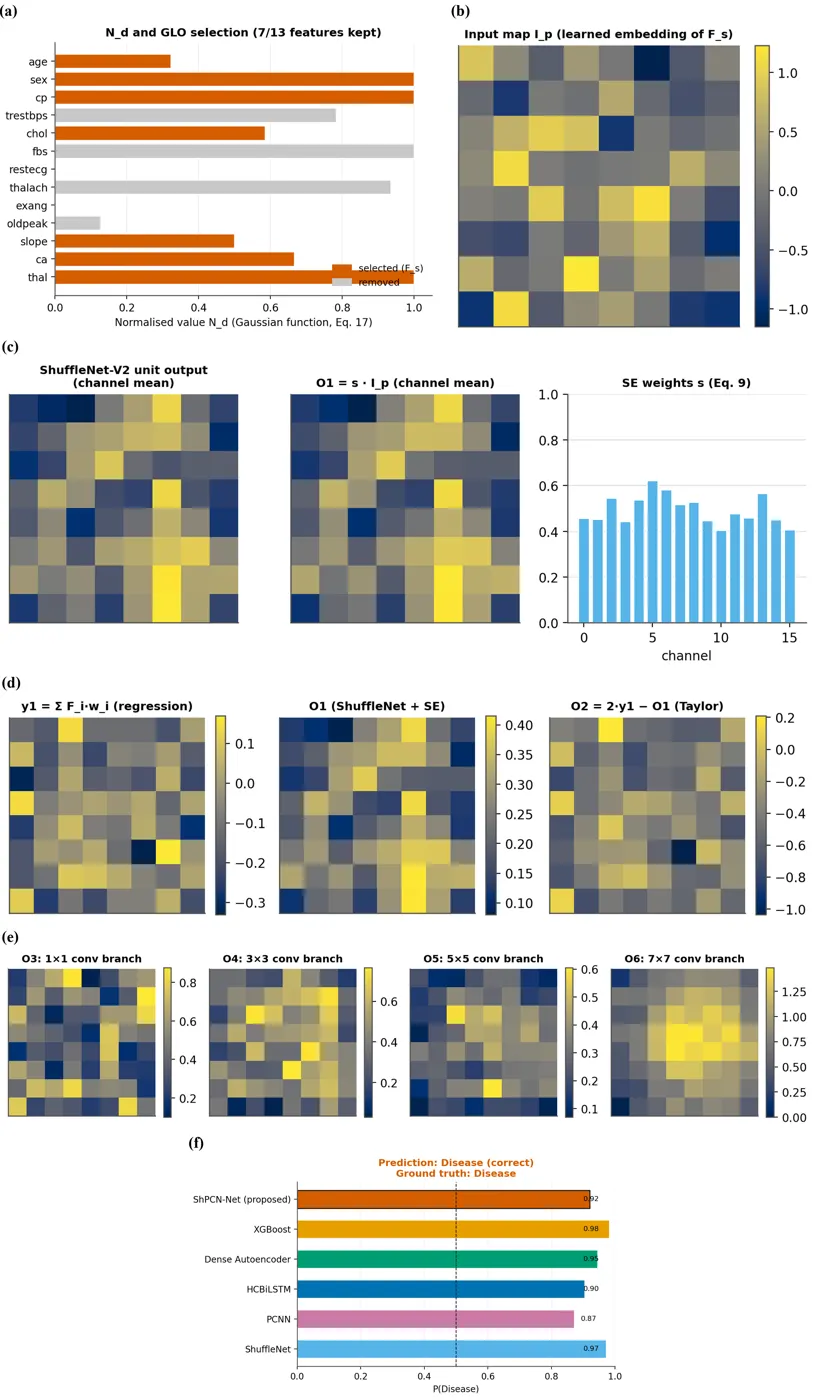
dataset: dataset_cleveland
sample_id: 21 (test sample of fold 1)
selected features (GLO): sex, cp, trestbps, thalach, slope, ca, thal
ShPCN-Net P(Disease) = 0.0324
predicted label: 0 (Normal)
ground truth   : 0 (Normal)

other methods P(Disease):
  ShuffleNet: 0.1355
  PCNN: 0.1273
  HCBiLSTM: 0.0838
  Dense Autoencoder: 0.0315
XGBoost: 0.0080代码在你自己的电脑上运行。所有文件、日志和结果都保存在项目文件夹里,没有任何隐藏。
- 记录数
- 303
- 验证方式
- 10 折交叉验证
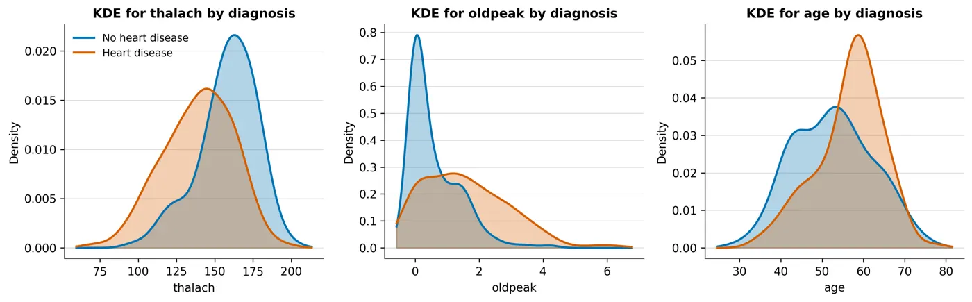
图片下方的文本文件是该记录保存的输出。
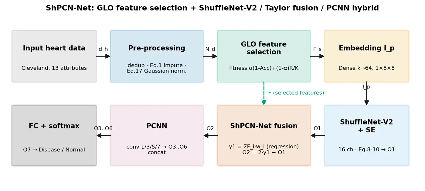
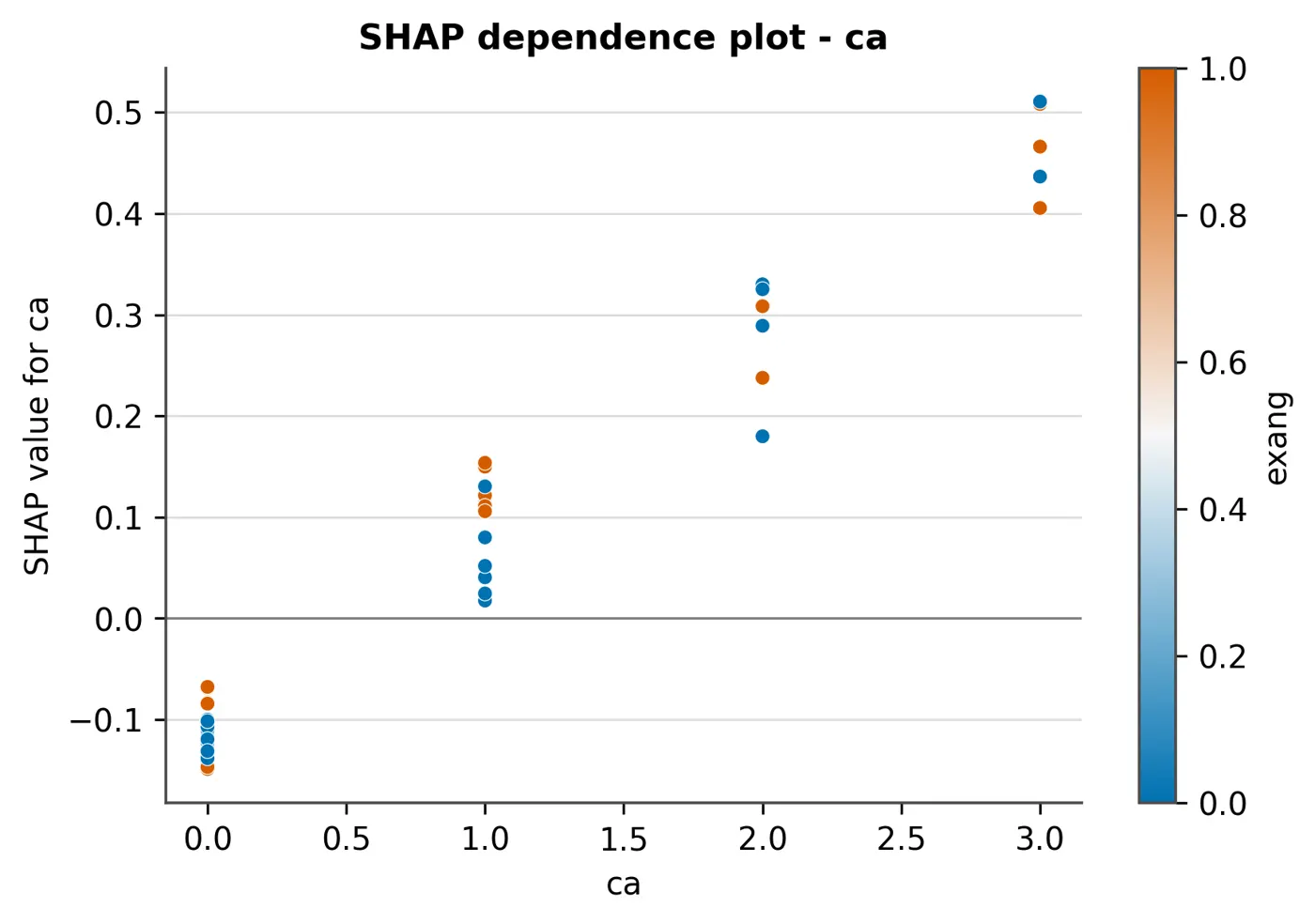
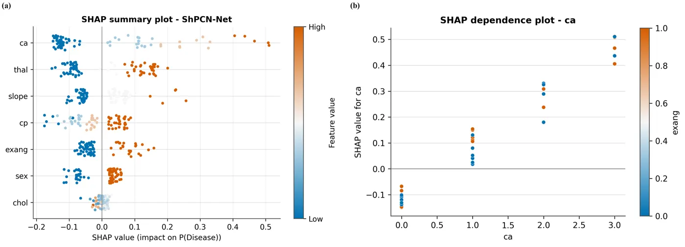
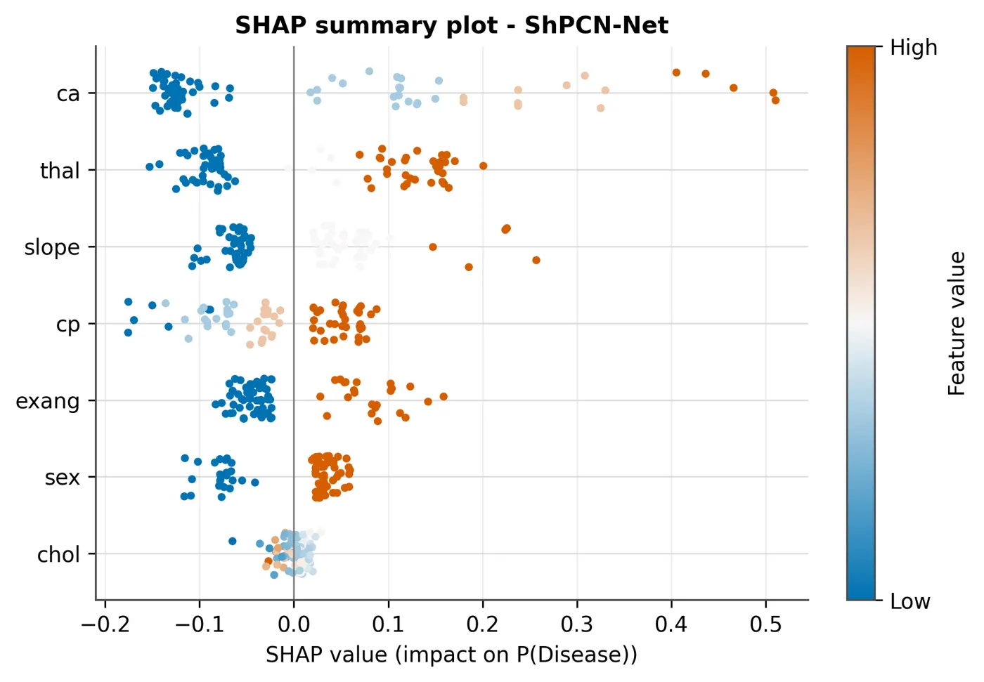
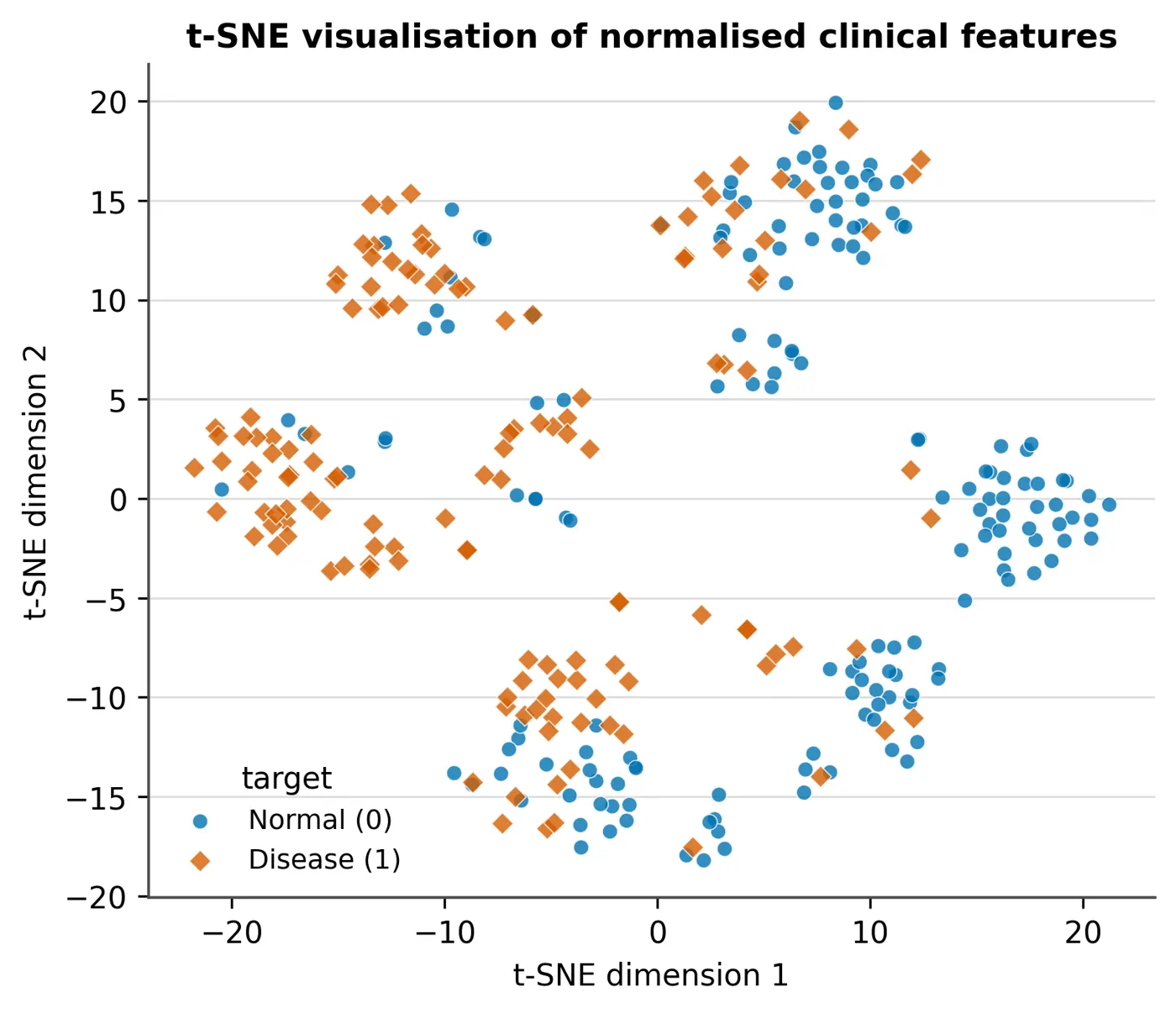
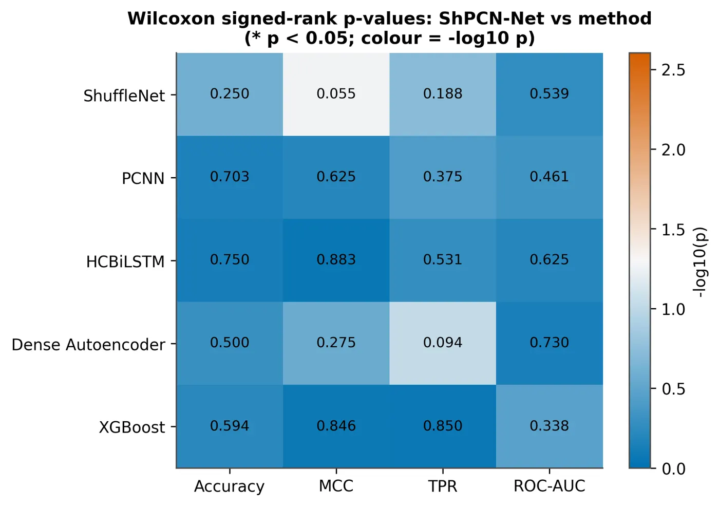
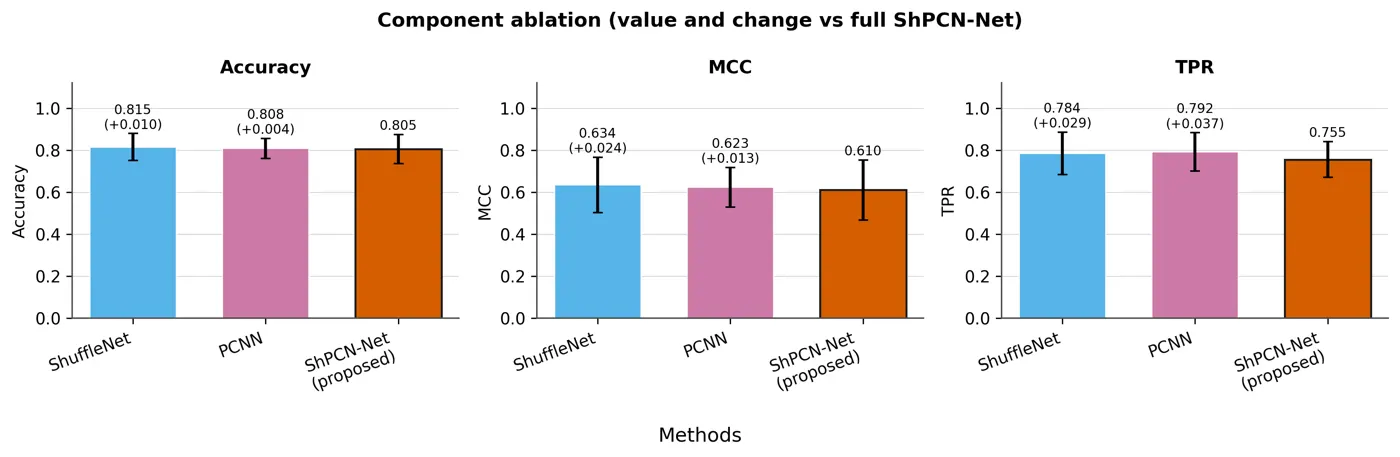
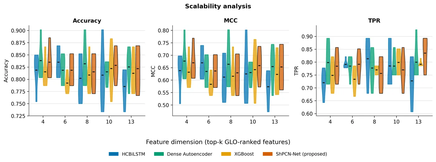
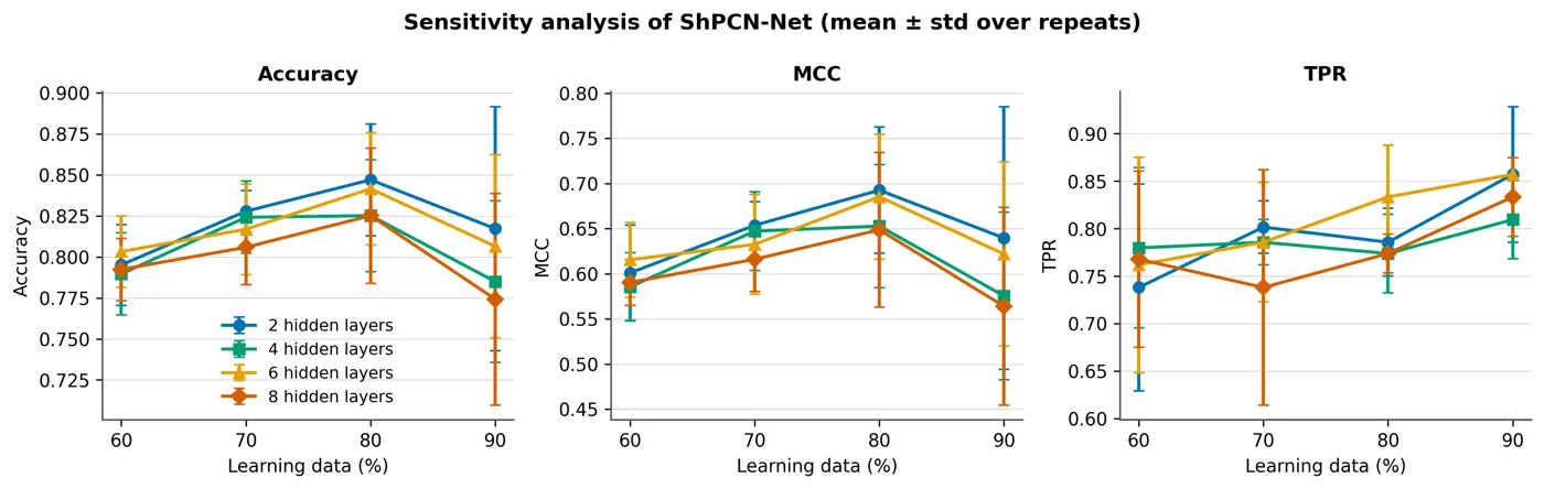
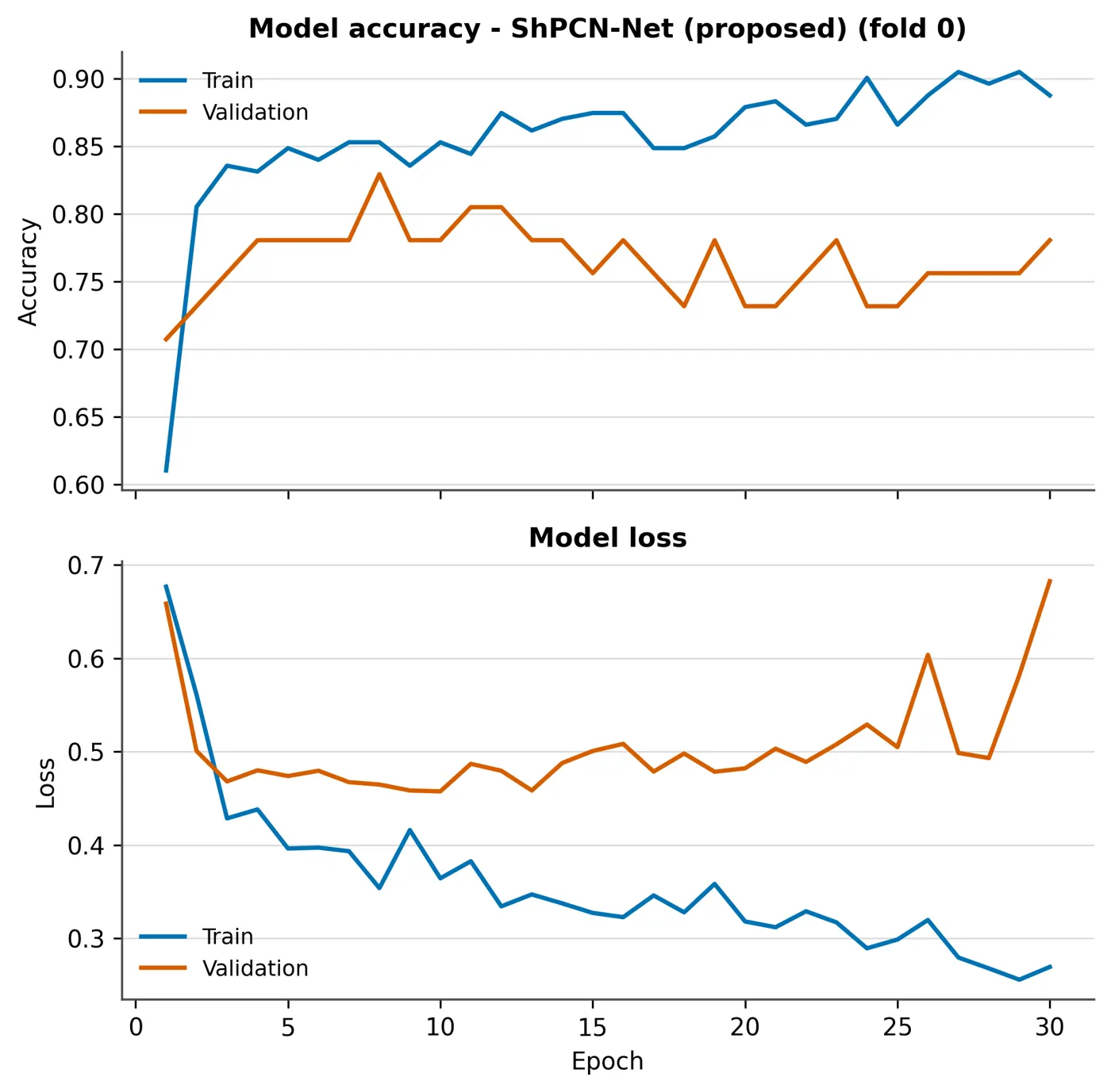
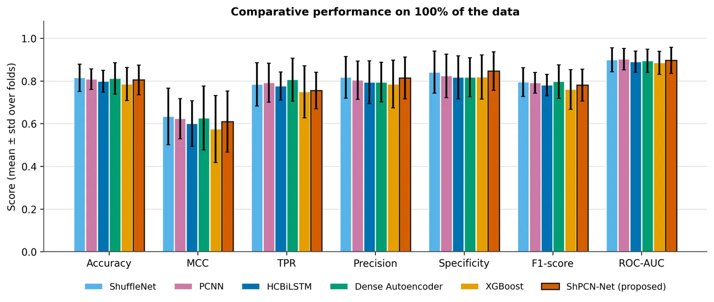
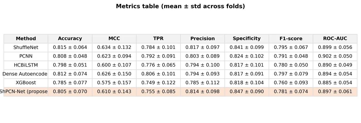
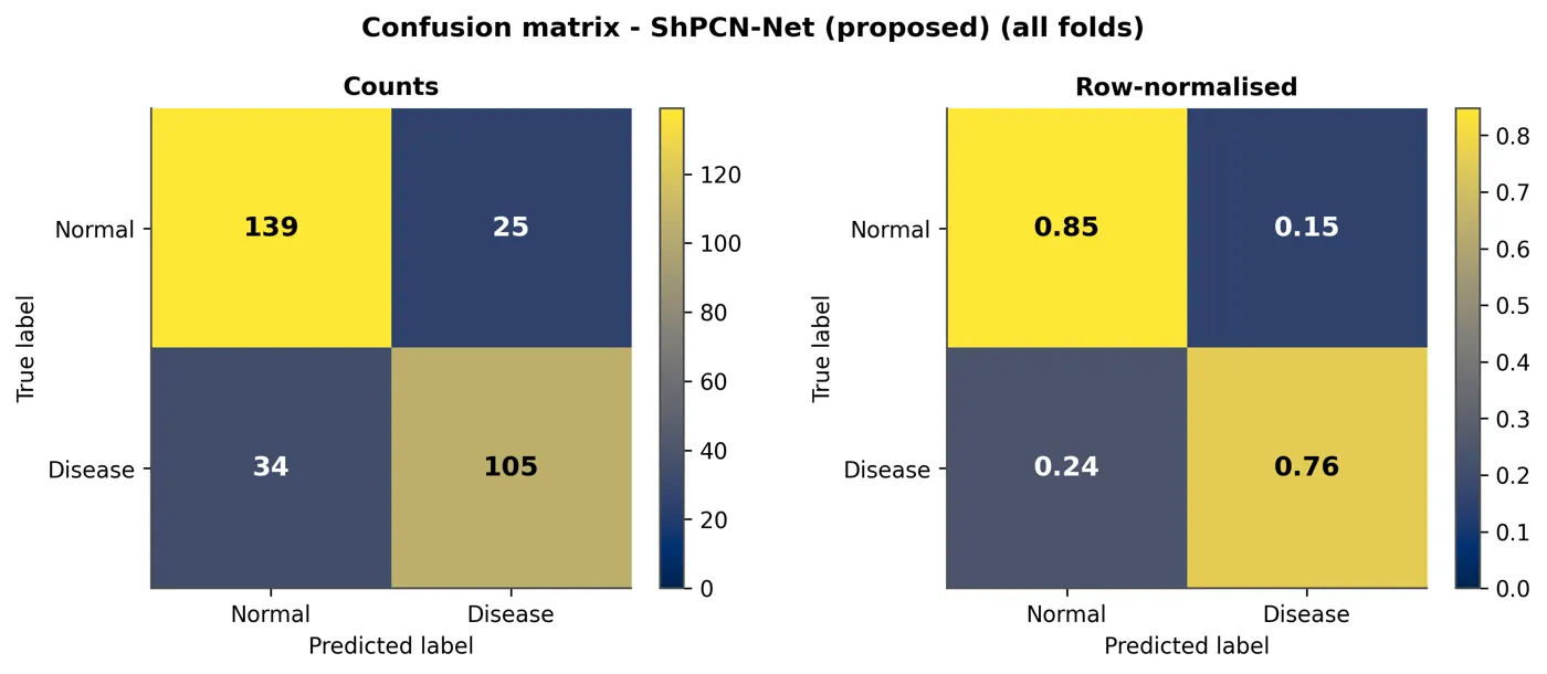
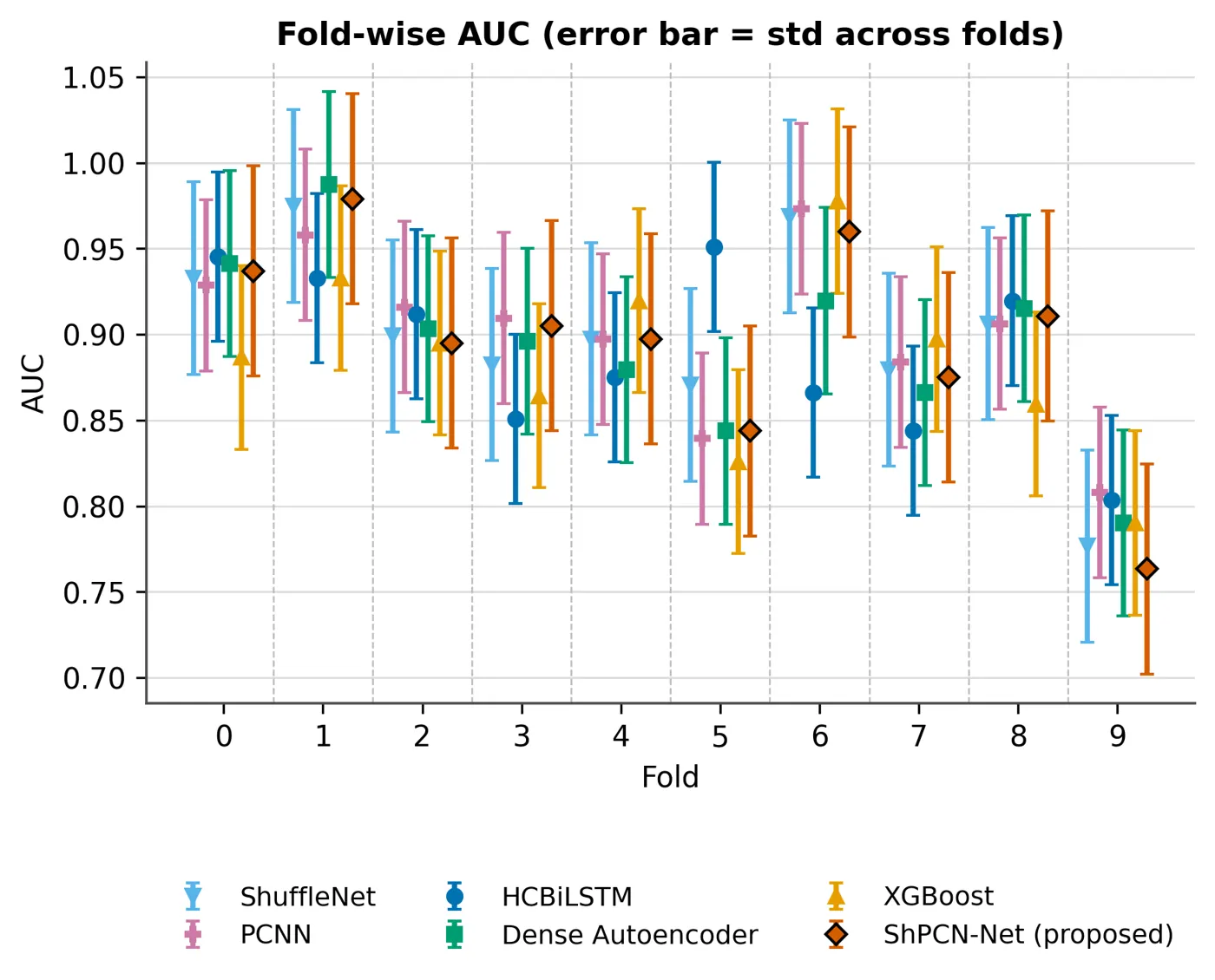
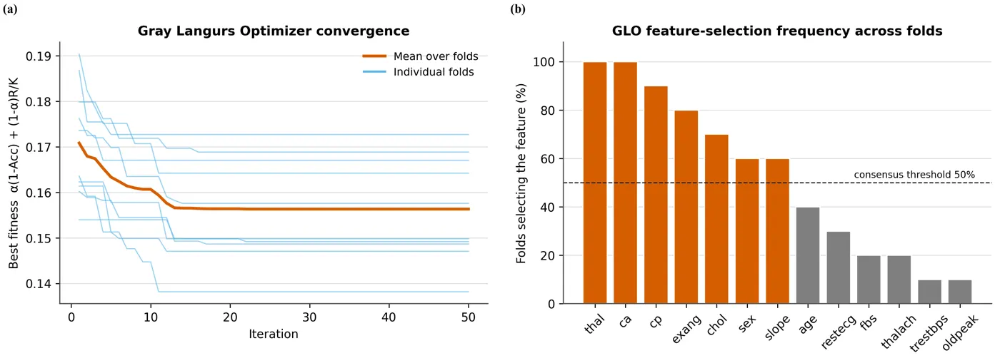
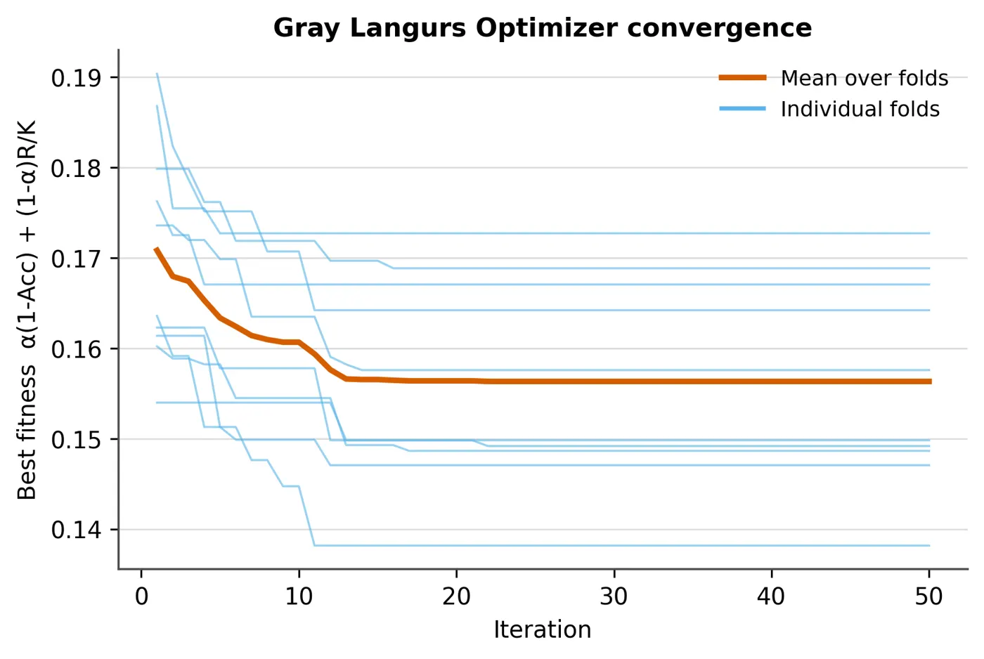
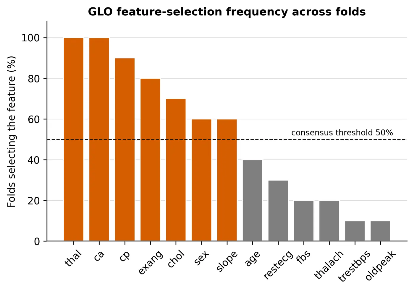
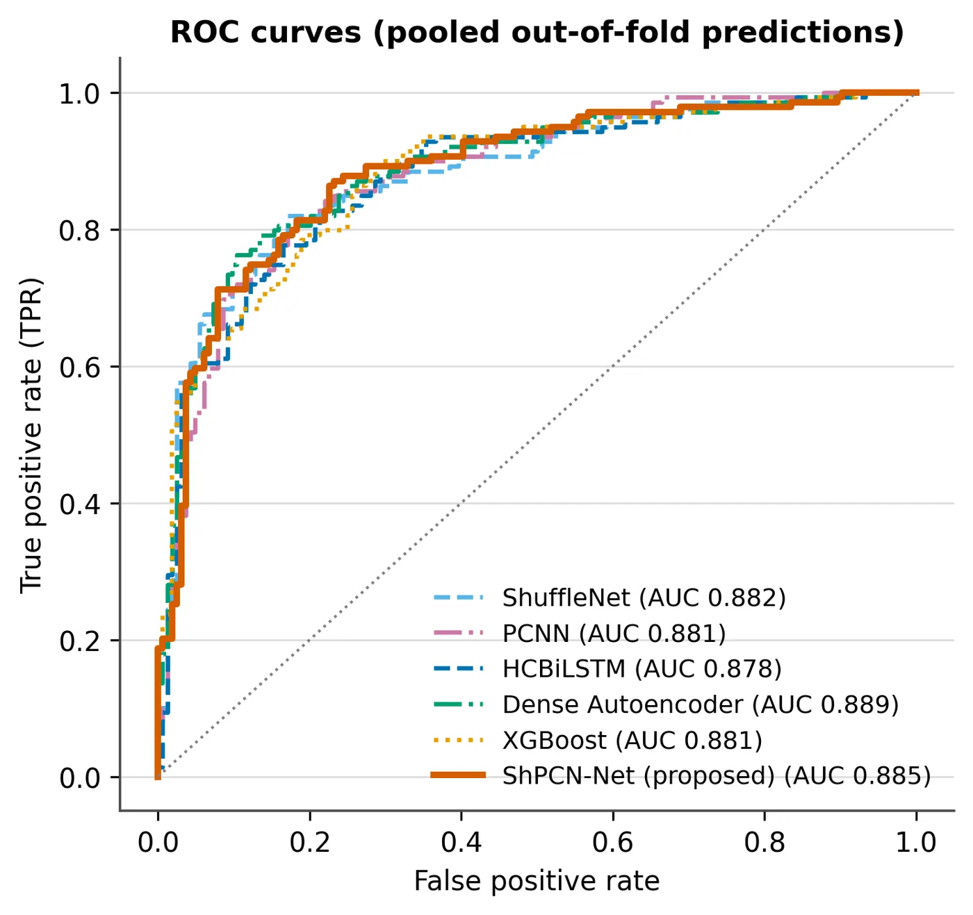
运行产生的每一张图表和示意图,按用途分组。可按组筛选,点击图表放大。
- 交付
- 22 张图表和示意图,全部展示
- 格式
- 每张图提供 PNG、矢量 PDF 和 CSV
正在加载 PDF… 0%
尚未做期刊排版的论文稿件,在 PDF 阅读器中查看,可跳页、缩放。
- 篇幅
- 34 页,排版前
- 阅读器
- 缩放、跳页、全屏、下载
正在加载 PDF… 0%
最终论文:同一份稿件按 IEEE 双栏版式排版,图表就位,参考文献已格式化。
- 最终论文
- 17 页,IEEE 双栏
- Word(DOCX)
- LaTeX 源文件
示例中的作者姓名均为占位符。
时间与成本
一篇论文能省下的小时和美元
以一篇期刊论文为例,分阶段估算:研究者在多个独立工具和付费支持之间来回工作,与在 EasySeer 中完成同样的工作相比。
| 研究阶段 | 研究者 + 现有工具* | EasySeer* |
|---|---|---|
| 构想与新颖性检查 | 10–20 小时 | 15–30 分钟 |
| 代码编写与调试 | 25–50 小时 | 30–90 分钟 |
| 代码运行与结果 | 15–30 小时 | 30 分钟–3 小时 |
| 论文稿件撰写 | 30–50 小时 | 30–90 分钟 |
| 排版与交付 | 5–10 小时 | 10–30 分钟 |
| 合计 | 105–200 小时 | 约 3–9 小时 |
105–200 小时 → 约 3–9 小时*
一个科研工作流可能节省 100 小时以上。
| 研究阶段 | 外部支持费用* | EasySeer* |
|---|---|---|
| 构想与新颖性检查 | 60–120 美元 | 已包含 |
| 代码编写与调试 | 150–300 美元 | 已包含 |
| 代码运行与结果 | 90–180 美元 | 已包含 |
| 论文稿件撰写 | 200–450 美元 | 已包含 |
| 排版与交付 | 40–90 美元 | 已包含 |
| 合计 | 630–1,380 美元 | 每个项目 100 美元 |
630–1,380 美元 → 每个项目 100 美元*
* 以一篇期刊论文估算。假设研究者经验中等,使用多个独立工具,成本部分假设每个阶段都购买外部付费支持。这些是 EasySeer 自己的规划估算,不是独立测得的结果,你的实际数字会有差异。
问题所在
为什么一篇论文要花 105–200 小时
时间很少花在科学本身上,而是耗在工具之间的衔接里。
工具分散
笔记一个工具,代码一个,写作一个,排版又一个。每次交接都要复制、重新解释、再修正。
发现太晚
想法不够新、缺少基线方法、与期刊不匹配,往往几个月后才发现,那时代码和初稿都已经写完。
结果无法追溯
稿件里的数字和产生它们的代码渐渐对不上,每次修改都得先花功夫去查。
EasySeer 把整个科研工作流放进同一个项目:想法、代码、结果、初稿和排版后的交付文件。每一步都由你批准。
对比
一条连贯的工作流,而不是一堆工具
通用 AI 助手适合很多工作。下面是它们用在这项工作上的一般情况。
适用人群
为用代码做研究并发表论文的人而设计
从一年级研究生到整个课题组,只要你要把一个想法、一些代码和一些数据变成论文,EasySeer 都适用。
博士研究生
多篇论文,一套工作流。尽早验证想法,所有文件放在一起。
了解更多 →硕士研究生
通过一个真实、有结构的项目,学会科研工作流。
了解更多 →博士后与青年研究者
在忙实验和基金申请的同时,更快把想法变成初稿。
了解更多 →导师
看到初稿背后的思路,把时间用在讨论科学问题上,而不是琐事。
了解更多 →工程与数据科学研究者
代码、日志、结果和文字放在一起,每个数字都能追溯到文件。
了解更多 →高校与课题组
让整个课题组使用同一套分步工作流,AI 使用声明也保持一致。
了解更多 →教师与讲师
在课程间隙,从一份已评分的构想开始写论文。
了解更多 →独立研究者
没有实验室或团队时,也有一套有结构的工作流。
了解更多 →企业研发团队
可复现的项目,数据留在你自己的电脑上。
了解更多 →医学与生命科学研究者
以代码驱动的研究,每一步都有记录。
了解更多 →使用非母语写作的研究者
基于你自己的结果,得到一份清晰的英文初稿。
了解更多 →科研管理部门与培训机构
一套可见的工作流,用来培训研究者。
了解更多 →- 你始终是作者EasySeer 只生成初稿。核实、改写和决定都由你来做。署名和责任属于你和你的合作者。
- 不编造数据结果来自在你的数据上真正运行过的代码。结果不理想,也如实呈现。
- 逐条核实参考文献建议的参考文献必须由你核对。有引用不等于结论成立。
- 声明 AI 的使用很多期刊和高校要求作者声明使用了 AI 辅助。EasySeer 帮你准备声明文字。请遵守适用于你的规定。
- 不承诺结果我们不承诺论文被录用,不承诺相似度数值,也不承诺检测工具会或不会标记文本。
- 每一步由你批准没有你的批准,流程不会往下走,你接受了什么都有清楚的记录。
EasySeer 是什么?
EasySeer 是一款 AI 科研工作流工具。从你的手写或打字输入的构想出发,它检查想法、编写代码、运行代码、撰写论文稿件、完成排版,并把结果交付到你的项目文件夹。
EasySeer 适合谁?
科研人员:博士和硕士研究生、博士后与青年研究者,以及导师和课题组。
EasySeer 会替我写论文吗?
不会。它只根据你提供的新颖构想生成初稿。内容需要你核实,并用你自己的语言改写,最终论文由你负责。
使用 EasySeer 符合学术伦理吗?
它按照学术伦理准则设计:如实报告结果,不编造数据,每一步都请你批准,并支持生成 AI 使用声明。请始终遵守你所在机构和期刊对 AI 辅助的规定。
EasySeer 能保证论文被期刊录用吗?
不能。录用由编辑和审稿人决定。EasySeer 不承诺录用、排名或任何相似度数值。
价格是多少?
每个项目 100 美元。1 点运行 1 个项目。
点数会过期吗?
不会。点数永不过期。
退款政策是什么?
已付款项不予退款。如果项目因我们这一方的故障失败,点数会退回;重复扣款或错误扣款会更正。详见退款政策。
面向顶尖研究水平
EasySeer 对标的标准
世界一流研究型大学的学者,对严谨和诚信有很高的要求。EasySeer 就是按这样的要求设计的。EasySeer 不声称与这里列出的任何大学有合作关系。
- 美国麻省理工学院
- 英国伦敦帝国理工学院
- 瑞士苏黎世联邦理工学院
- 新加坡新加坡国立大学
- 中国香港特别行政区香港大学
- 澳大利亚新南威尔士大学(悉尼)
- 德国慕尼黑工业大学
- 加拿大麦吉尔大学
- 法国巴黎文理研究大学
- 韩国首尔国立大学